3 The pipeline
The code and prose in this book were written by Claude Code (an AI coding agent) under human direction. They have not been line-by-line verified by a human and must not be published or cited as-is.
These are exploratory analyses of preliminary, in-progress work. Results and numbers have not been independently reviewed or validated and require checking before any use.
This chapter walks through the whole modeling pipeline, from raw cluster data to a trained model and its evaluation. The design goal is iteration speed: every choice below is made so that a full experiment runs in minutes, letting us test many hypotheses about the learning signal rather than one expensive model.
3.1 Data on the cluster
Chapter 2 describes the corpus itself (scale, speech, annotations); this section is just the on-cluster asset layout the pipeline reads. Everything derives from the BabyView 2025.2 release on ccn2, under /ccn2a/dataset/babyview/2025.2/:
| Asset | What it is | Used for |
|---|---|---|
extracted_frames_1fps/<video>/NNNNN.jpg |
video frames at 1 fps (8,566 videos) | vision input |
outputs/merged_transcripts_parsed.csv |
4.56M token rows, WhisperX + spaCy POS/lemma | text input, filtering |
outputs/full_clip_results.csv |
1.28M utterances with per-utterance frame–utterance CLIP scores | the alignment filter |
outputs/object_detections/cdi/<video>/ |
YOLOE detections prompted with the CDI noun list (2,969 videos) | evaluation + region grounding |
A single utterance, then, is a row with a video, a start/end time, the words spoken, and a precomputed CLIP alignment score. Frames are a dense 1 fps extraction of every video (5.42M frames; every second of every recording, not a pre-selected subset), and each utterance is paired with the frame at its temporal midpoint. At 1 fps a frame index is just a timestamp in seconds, so this is a pure timestamp lookup: no alignment score — CLIP or otherwise — plays any role in which frame an utterance gets.1
3.2 The alignment filter
The filter is the central knob. The cheap version — used in the preliminary experiments — reads full_clip_results.csv, which stores for each utterance the maximum CLIP cosine similarity between its text and any frame in its window (clip_score_max). Selecting above a threshold costs nothing and, as Figure 3.1 shows, separates grounded from ungrounded moments. The main chapters instead use the stronger Gemini annotation of Chapter 2 as the gold definition of alignment (and its referent word as the gold label), keeping CLIP as the weaker comparison; the mechanics below are identical either way.
Building a training manifest is then one pass over the CSV with a threshold, a held-out child excluded, and (optionally) a size cap for size-matched controls:
# src/build_pairs.py (abridged)
df = pd.read_csv(CLIP_RESULTS)
df = df[df.clip_score_max >= args.min_clip]        # the alignment knob
df = df[~df.child_id.isin(held_out)]               # cross-child generalization
df["frame_idx"] = ((df.start + df.end) / 2).astype(int)   # midpoint frame
3.3 The vision tower: frozen DINOv2
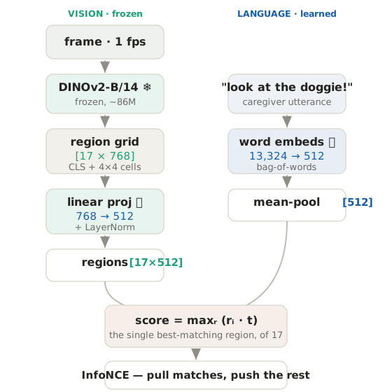
Each frame is embedded once by a frozen DINOv2-base encoder (a self-supervised Vision Transformer) into a 768-dimensional vector — the model’s pooler_output (the CLS token). We compute these embeddings for every frame any experiment needs (~1.27M frames) and cache them to disk as float16 (~1.5 KB per frame). Nothing about the vision encoder is learned.
Freezing the vision tower is the decision that makes the prototype fast and the experiments clean:
- Fast. With frames precomputed, a training run reads 768-d vectors and fits only a small projection and word embeddings — minutes on one GPU.
- Clean. Because capacity and optimization are held fixed, differences between runs reflect which pairs the model sees, not how hard the vision problem is. (This also means our probe cannot reproduce the training-loss divergence reported for end-to-end pixel models — but it isolates the alignment effect that divergence obscures.)
3.4 The text tower: bag of words
Following CVCL’s finding that architecture barely matters, the text encoder is deliberately minimal: an embedding table over the training vocabulary, mean- pooled across the tokens of an utterance. A word’s meaning is just its embedding; an utterance’s meaning is the average of its words’.
3.5 The joint space and the contrastive objective
Both towers project to a shared \(d\)-dimensional space and are L2-normalized. For a batch of \(N\) (image, text) pairs with embeddings \(v_i\) and \(t_i\), cosine similarities are scaled by a learned temperature \(\tau\) and trained with the symmetric InfoNCE loss — each image should pick its own caption out of the batch, and vice versa:
\[ \mathcal{L} = \tfrac12\!\left[ -\frac1N\sum_i \log\frac{e^{s\,\langle v_i,t_i\rangle}}{\sum_j e^{s\,\langle v_i,t_j\rangle}} \;-\;\frac1N\sum_i \log\frac{e^{s\,\langle v_i,t_i\rangle}}{\sum_j e^{s\,\langle v_j,t_i\rangle}} \right], \qquad s = 1/\tau. \]
The whole model is about thirty lines:
# src/train.py — the two-tower model
class TwoTower(nn.Module):
    def __init__(self, vocab_size, dim=512, drop=0.1):
        super().__init__()
        self.vproj = nn.Sequential(nn.LayerNorm(768), nn.Dropout(drop),
                                   nn.Linear(768, dim))          # frozen-emb -> joint
        self.word = nn.Embedding(vocab_size, dim, padding_idx=0) # bag of words
        self.logit_scale = nn.Parameter(torch.tensor(np.log(1/0.07)))

    def encode_image(self, v):
        return F.normalize(self.vproj(v), dim=-1)

    def encode_text(self, t, n):
        e = self.word(t)                                # [B, L, D]
        mask = (t != 0).unsqueeze(-1).float()
        pooled = (e * mask).sum(1) / n.clamp(min=1).unsqueeze(-1)
        return F.normalize(pooled, dim=-1)

    def forward(self, v, t, n):
        iv, tv = self.encode_image(v), self.encode_text(t, n)
        logits = self.logit_scale.clamp(max=np.log(100)).exp() * iv @ tv.t()
        labels = torch.arange(len(v), device=v.device)
        return 0.5 * (F.cross_entropy(logits, labels) +
                      F.cross_entropy(logits.t(), labels))
Defaults: joint dim 512, batch 256, AdamW at lr \(3\times10^{-4}\), 20 epochs, vocabulary of words appearing \(\ge 5\) times.
It is worth being explicit about how little is trained. The vision encoder is frozen, so the entire learned image→joint map is one LayerNorm plus a single \(768\times512\) linear — about 0.4M parameters. Everything else is the word table (vocabulary \(\times\,512\): a few million parameters for a vocabulary of a few thousand words) and one scalar temperature. There are no learned vision parameters; “alignment” here is literally a linear projection of frozen DINOv2 features, a bag-of-words lookup table, and a temperature. That thinness is deliberate — it isolates the alignment signal from encoder capacity — and it is what makes the label topline of Chapter 4 interpretable: when this map reaches its ceiling under clean labels, what we are measuring is the frozen features’, not the probe’s.
3.6 Training dynamics: what the loss does
Because the model is so small and the features are precomputed, training is fast and its dynamics are clean. All arms drive the training loss down at similar rates — the linear map and word table can always fit the pairs they are given. What separates them is the held-out contrastive loss, and it separates them sharply (held-out child S00360001, seed 0):
| training arm | pairs | train loss (ep 0→19) | val loss | best 4AFC (epoch) | val-loss behavior |
|---|---|---|---|---|---|
| aligned (clip>0.24) | 137k | 5.38 → 3.70 | 5.21 → 4.97 (min ep 6) → 5.10 | 46.7 (ep 7) | dips, then drifts up mildly |
| unfiltered (everything) | 1.14M | 5.46 → 4.48 | 5.39 → 5.13, then flat | 43.2 (ep 7) | falls, never rises |
| random (size-matched) | 137k | 5.56 → 4.40 | 5.46 → 5.79 | ~34 (flat) | climbs steadily — overfits |
Three things follow, and they recur throughout the book:
- The held-out loss, not the training loss, is the quality signal. Random pairs overfit hard — train loss falls normally while val loss climbs monotonically — because there is no generalizable frame↔︎text structure to find, so the model memorizes. Aligned pairs generalize: val loss dips and then only drifts up slightly. The gap between these two curves is the alignment effect, visible before any 4AFC number.
- Accuracy converges in well under ten passes. 4AFC peaks around epoch 6–8 everywhere and the val-loss minimum roughly coincides, so we report the best epoch; early stopping would not change any conclusion. Twenty epochs is generous headroom, not a tuned stopping point.
- Our frozen probe does not reproduce end-to-end “divergence.” The unfiltered 1.14M arm’s val loss falls and flattens (5.39 → 5.13) — it never rises. The loss-climbing reported for full end-to-end BabyView contrastive training is therefore an optimization/capacity effect layered on top of the alignment problem; the probe deliberately strips it away, so our claim is “filtered > unfiltered,” not “unfiltered diverges.”
3.7 Evaluating: the Konkle 4AFC test
We evaluate on out-of-sample objects, not held-out frames. The primary metric is a 4AFC test on the Konkle object benchmark — clean photographs of everyday objects on white backgrounds, entirely disjoint from BabyView. A trial presents a cue word and four object images (one from the cue’s category, three from other categories); the model picks the image whose embedding is closest to the word embedding. Chance is 25%.
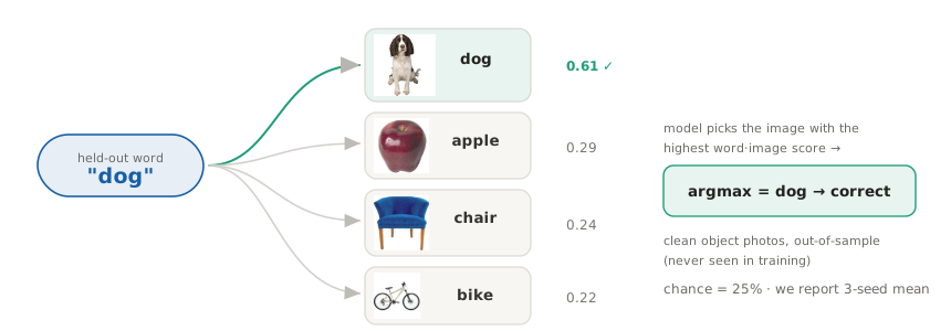
Evaluating on external objects has three virtues. It is truly out of sample — no BabyView frame appears in it — so we can train on the entire corpus, all 36 children, with no leakage, and the held-out-child machinery of the appendices becomes unnecessary. It is clean — the noisy, detector-derived ground truth of the naturalistic eval below compressed real effects into noise (the same interventions move ~2–3× more on Konkle). And it mirrors a fact about children: they recognize objects they have never seen in that exact form, so generalization to canonical exemplars is the right target, not memorization of frames.
Dev/test split. The full Konkle set has ~200 categories; Vong et al. (2024)’s subset of 60 is our test set, and the other 118 in-vocabulary categories form a dev set on which we tune any hyperparameter (filter thresholds, cue weights), reporting final numbers on the Vong-60. A clean, out-of-sample split that keeps the sweeps honest.
The legacy naturalistic eval. The preliminary experiments (appendices) instead used a 4AFC over held-out BabyView frames, each labeled by its dominant CDI-prompted YOLOE detection (largest, confident, a clear majority of detected object area). It needs no human annotation and runs every epoch, and it is retained as a secondary signal — but it is noisy and detector-biased, so the clean Konkle eval is primary throughout the main chapters.
3.8 The three bootstrapping mechanisms
The alignment filter attacks when to learn. The learner also has to decide what to attend to within a learning moment — and it can try to do so without being told the answer, i.e. by self-supervised selection. Three mechanisms operate at different grains; Chapter 4 measures what each buys:
- Region MIL — where in the frame. Embed a coarse grid of image cells (a \(4\times4\) grid plus the whole-frame token, 17 vectors) and score the utterance against its best-matching cell — a max over cells, i.e. multiple-instance learning. The frame is a bag of regions; the utterance is assumed to match at least one. This does implicit referent localization with no detector, and it is the single largest free gain in the book.
- Frame MIL — which moment. Extend the max over the frames in a short window (±2 s) around the utterance, so the model can pick the moment that best shows the referent.
- Utterance EM — which pairs. Reweight the training pairs by the model’s own estimate of alignment (its max-region similarity) in an EM loop: better weights → better model → better weights. This is the self-supervised attempt to recover the alignment filter without an oracle.
All three share the same frozen DINOv2 features and contrastive objective; they differ only in what the utterance is allowed to match. Earlier experiments used a hard-coded detector crop as a stand-in for region grounding; region MIL replaces it.
3.9 Reproducing
The pipeline is a handful of small scripts, run on ccn2 with the environment at /data2/mcfrank/ladder/condaenv:
python build_eval.py    --videos held_out_child_videos.txt   # labeled 4AFC frames
python build_pairs.py   --name aligned --min-clip 0.24 ...    # training manifest
python embed_frames.py  --frames frames_all.parquet           # cache DINOv2 features
python train.py         --manifest aligned.parquet ...        # train + eval
Frame embeddings and run logs live under /data2/mcfrank/vlm-headcam/; only aggregate results are committed to the repository (human-subjects frames stay on the cluster).
Verified directly: in 300 randomly sampled videos, frame indices run contiguously
00000…N−1with no gaps, and the last index matches the last utterance time. The frame tree (extracted 2025-09) also predatesfull_clip_results.csv(2025-10), whose per-utteranceclip_score_min/mean/maxwere computed over these dense frames.↩︎