6 Scaling and data distribution
The code and prose in this book were written by Claude Code (an AI coding agent) under human direction. They have not been line-by-line verified by a human and must not be published or cited as-is.
These are exploratory analyses of preliminary, in-progress work. Results and numbers have not been independently reviewed or validated and require checking before any use.
Chapter 2 showed the corpus is large but extremely uneven across children. This chapter asks why the numbers are where they are along two axes — how much data, and whose — using the region-MIL learner on subsamples of the 911k training pairs, all evaluated on Konkle test-60 (3 seeds), redoing on the clean eval an analysis we first ran with CLIP-era tooling.
6.1 How much data
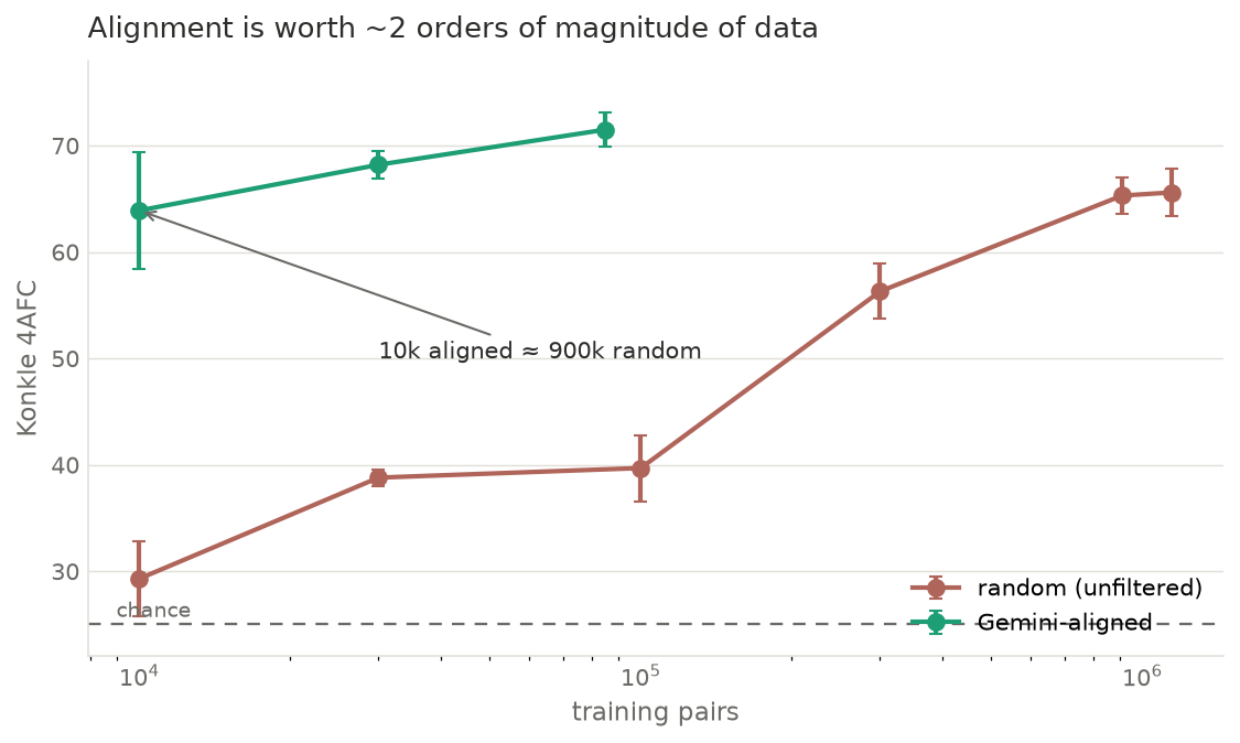
We compare two scaling curves: random (unfiltered) subsamples, and the Gemini-aligned top-N pairs, across training-set sizes.
| pairs | random | aligned |
|---|---|---|
| 10k | 30.0 ± 3.5 | 63.9 ± 5.5 |
| 30k | 38.3 ± 0.8 | 68.0 ± 1.3 |
| 85k | — | 71.4 ± 1.6 |
| 100k | 40.2 ± 3.1 | — |
| 300k | 56.2 ± 2.6 | — |
| 911k | 65.3 ± 1.7 | — |
| 1.14M (full corpus) | 65.6 ± 2.2 | — |
Two findings. First, contrary to the natural guess, the random baseline does not plateau — it climbs from chance-ish to 65.6 across the range and is still rising even at the full corpus (adding the held-out 20% to the 911k lifts it another +3). This full-corpus model is the definitive best-organic learner interpreted in Chapter 7. Unfiltered training is genuinely data-limited: because most pairs are non-referential noise, the model needs a great deal of data to average out. Second, and this is the headline, alignment is worth ~2 orders of magnitude of data: 10k aligned pairs (63.9) already match ~900k random ones (65.3), and the aligned curve is near the label ceiling by 85k. So the lever is not “more data” in the absolute — it is concentration: a few tens of thousands of aligned pairs beat a million unfiltered ones.
(One caveat: at the smallest sizes the low-vocabulary runs cover fewer of the 60 Konkle categories, so the absolute low-N numbers are dragged toward chance and the aligned/random comparison there is not category-matched; the ~30-point gap at every count is robust regardless.)
6.2 Across developmental time
The alignment-efficiency result invites a developmental reading. Converting the x-axis from training pairs to hours of experience — at roughly 820 utterances per hour in this corpus, and the conventional 4,000 hours per year — and extrapolating the fitted saturating curves lets us ask what these scaling laws imply across years of a child’s life.
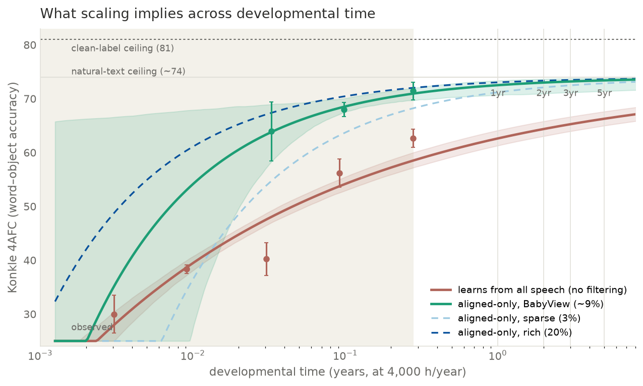
Three things stand out. First, filtering is worth years of developmental time: a learner that could perfectly concentrate the aligned moments (green) reaches the natural-text ceiling within about a year, while the unfiltered learner (red) is still climbing toward it after five. Second, the intrinsic alignment density of a child’s environment matters: a corpus with more referential talk (rich, 20%) reaches high accuracy roughly a year ahead of a sparse one (3%). Third, everyone converges toward the same natural-text ceiling (~74) — noiseless labels (81) would add more, but real speech does not provide them.
Two honesty caveats. The curves right of the “observed” region are extrapolation from a saturating fit, so the year-scale numbers are illustrative, not predictions. And the aligned curves are oracles — Chapter 5 showed a child cannot actually perform this filtering, so they mark the value of an alignment-selection ability we could not supply; the achievable trajectory is the red one. The developmental moral is not that this model learns like a child, but that referential alignment sets the timescale: how fast word–object mapping comes online is governed less by how much a child hears than by how much of it is about something they can see.
6.3 Whose data
Holding the amount fixed, does it matter whose data it is?
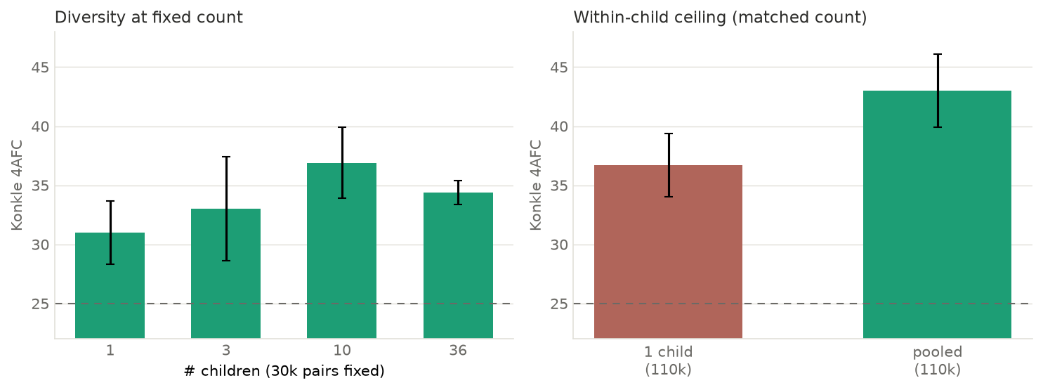
The clean comparison is the within-child ceiling: the biggest single child contributes 110k pairs, and trained on those alone the model reaches 36.7 ± 2.7; a pooled random sample of the same 110k count reaches 43.0 ± 3.1 — +6 for diversity at matched amount. One child’s world, even a large one, hits a low ceiling that pooling across homes clears. The finer sweep — fixing 30k pairs and varying the number of contributing children (1 → 36) — points the same way (31.7 → ~35) but is within seed noise, so we read diversity as a real but moderate effect, not a dominant one.
6.4 Synthesis
The corpus is both data-limited and signal-limited, and the resolution for both is the same: concentrate aligned data from many children. Alignment buys ~90× data efficiency; diversity buys ~+7 at matched count. Neither raw volume from one child nor unfiltered volume from many is the answer — the useful signal is aligned, referential moments, sampled broadly. This is the data-side complement to the mechanistic story of Chapter 4: the bottleneck is the quality and breadth of the referential signal, not the amount of raw experience.