source(here::here("common.R"))
library(lme4)
library(broom.mixed)
library(ggrepel)

scores_all <- read_rds(here("data", "scores_all_sites.rds"))02 — Longitudinal traces and simple growth models
ImportantAI-generated — not for publication
The code and prose in this chapter were written by Claude Code (an AI coding agent) under human direction. They have not been line-by-line verified by a human and must not be published or cited as-is.
WarningPreliminary & unvetted analysis
These are exploratory analyses of preliminary, in-progress LEVANTE data. Results have not been reviewed or validated and require checking by the LEVANTE Data Coordinating Center before any use.
NoteNow on corrected data (v1.2)
Re-run on levante_data_latest v1.2, which fixes the IRT column-order scoring bug. The spurious within-child declines seen in earlier (v1.0) renders are gone: all within-child slopes are now positive (e.g. Math ≈ 0.6 θ/yr, Vocab/EF/reasoning ≈ 0.1–0.4). Any text below that frames a task as “declining” reflects the old buggy data and is superseded by the corrected figures.
Note2026-08 data update: rural Colombia’s second wave
The 2026-08 snapshot adds Caquetá/Boyacá as a fourth longitudinal dataset (~213 repeat kids at a ~9.6-month gap, concentrated in ROAR + Math). Its within-child growth is clean and — notably — almost exactly matches the cross-sectional age gradient: Math 0.45 θ/yr within vs 0.45 across, ROAR-Word 0.47 vs 0.49, ROAR-Phoneme 0.28 vs 0.28, ROAR-Sentence 0.22 vs 0.23. Math repeats are CAT→CAT (no mode transition), making this the cleanest within-child growth replication in the project so far.
2026-08-31: Leipzig’s third wave began arriving (39 children re-tested on the full battery Aug 29–30, already scored in the draft snapshot) — the first ≥3-timepoint children in the project. They appear in the Leipzig spaghetti below as three-point trajectories (max within-child span now 24 months); per-child growth-curve models become identifiable once this wave completes.
Purpose
00 inventoried what data we have; 01 audited per-(site, task) data integrity and produced a verdict table at data/task_site_verdict.rds. This notebook focuses on the datasets that actually have repeat assessments and asks:
- Do individual children show consistent growth in IRT ability scores across waves?
- Are within-individual growth rates broadly consistent with the cross-sectional age gradient in that dataset?
We restrict attention to the four datasets with meaningful longitudinal signal as of the 2026-08 per-site snapshot:
- Germany — Leipzig (mpieva-de): ~3- and 7-month retest, ~226 kids.
- Colombia — Bogotá (uniandes-co-bogota): ~15-month gap, ~420 kids.
- Colombia — Caquetá/Boyacá (uniandes-co-rural): new in the 2026-08 update — a ~9.6-month-gap second wave, ~213 repeat kids. Repeats are concentrated in ROAR (pa/swr/sre) and Math (~170–210 pairs each; Math is cleanly CAT→CAT); the other core tasks are still cross-sectional here.
- Canada — Ontario (western-ca): ~12-month gap, still only ~10–21 repeat kids per task, so it falls below the ≥ 30-per-task threshold for the mixed models and mainly appears in the spaghetti/cross-sectional views.
Restrict to longitudinal datasets
long_datasets <- c("pilot_mpieva_de_main",
                   "pilot_uniandes_co_bogota",
                   "pilot_uniandes_co_rural",
                   "pilot_western_ca_main")

scores <- scores_all |>
  filter(dataset %in% long_datasets,
         !is.na(score), !is.na(age))

scores |>
  count(dataset_label, task_label) |>
  pivot_wider(names_from = dataset_label, values_from = n,
              values_fill = 0L) |>
knitr::kable()| task_label | Colombia — Bogotá | Colombia — Caquetá/Boyacá | Germany — Leipzig | Canada — Ontario |
|---|---|---|---|---|
| Hearts and Flowers | 435 | 491 | 564 | 398 |
| Math | 908 | 1182 | 534 | 370 |
| Memory | 344 | 485 | 539 | 361 |
| Pattern Matching | 327 | 468 | 506 | 299 |
| ROAR-Phoneme | 578 | 1162 | 0 | 292 |
| ROAR-Sentence | 769 | 936 | 198 | 126 |
| ROAR-Word | 787 | 1007 | 203 | 140 |
| Same and Different | 204 | 230 | 542 | 267 |
| Sentence Understanding | 454 | 601 | 439 | 346 |
| Shape Rotation | 410 | 536 | 474 | 345 |
| Stories (ToM) | 190 | 304 | 525 | 254 |
| Vocabulary | 336 | 651 | 524 | 348 |
Adaptive vs non-adaptive scores
Pilot data mixes non-adaptive and computer-adaptive (CAT) administrations of the same task. Under v1.0’s scoring bug this produced large spurious step jumps across the mode boundary; on v1.2 (fixed) the residual mode shift is small (< 0.75 logits — see 01), attributable to mild ceiling on the easy non-adaptive forms plus EAP shrinkage. We still flag the mode split below so within-mode vs across-mode comparisons stay visible.
scores |>
  group_by(dataset_label, task_label, adaptive) |>
  summarise(n_runs = n_distinct(run_id), .groups = "drop") |>
  pivot_wider(names_from = adaptive, values_from = n_runs, values_fill = 0L,
              names_prefix = "adaptive_") |>
knitr::kable()| dataset_label | task_label | adaptive_FALSE | adaptive_TRUE |
|---|---|---|---|
| Colombia — Bogotá | Hearts and Flowers | 435 | 0 |
| Colombia — Bogotá | Math | 331 | 577 |
| Colombia — Bogotá | Memory | 344 | 0 |
| Colombia — Bogotá | Pattern Matching | 81 | 246 |
| Colombia — Bogotá | ROAR-Phoneme | 578 | 0 |
| Colombia — Bogotá | ROAR-Sentence | 769 | 0 |
| Colombia — Bogotá | ROAR-Word | 787 | 0 |
| Colombia — Bogotá | Same and Different | 166 | 38 |
| Colombia — Bogotá | Sentence Understanding | 177 | 277 |
| Colombia — Bogotá | Shape Rotation | 338 | 72 |
| Colombia — Bogotá | Stories (ToM) | 151 | 39 |
| Colombia — Bogotá | Vocabulary | 63 | 273 |
| Colombia — Caquetá/Boyacá | Hearts and Flowers | 491 | 0 |
| Colombia — Caquetá/Boyacá | Math | 220 | 962 |
| Colombia — Caquetá/Boyacá | Memory | 485 | 0 |
| Colombia — Caquetá/Boyacá | Pattern Matching | 23 | 445 |
| Colombia — Caquetá/Boyacá | ROAR-Phoneme | 1162 | 0 |
| Colombia — Caquetá/Boyacá | ROAR-Sentence | 936 | 0 |
| Colombia — Caquetá/Boyacá | ROAR-Word | 1007 | 0 |
| Colombia — Caquetá/Boyacá | Same and Different | 20 | 210 |
| Colombia — Caquetá/Boyacá | Sentence Understanding | 53 | 548 |
| Colombia — Caquetá/Boyacá | Shape Rotation | 0 | 536 |
| Colombia — Caquetá/Boyacá | Stories (ToM) | 91 | 213 |
| Colombia — Caquetá/Boyacá | Vocabulary | 76 | 575 |
| Germany — Leipzig | Hearts and Flowers | 564 | 0 |
| Germany — Leipzig | Math | 430 | 104 |
| Germany — Leipzig | Memory | 539 | 0 |
| Germany — Leipzig | Pattern Matching | 434 | 72 |
| Germany — Leipzig | ROAR-Sentence | 198 | 0 |
| Germany — Leipzig | ROAR-Word | 203 | 0 |
| Germany — Leipzig | Same and Different | 434 | 108 |
| Germany — Leipzig | Sentence Understanding | 192 | 247 |
| Germany — Leipzig | Shape Rotation | 189 | 285 |
| Germany — Leipzig | Stories (ToM) | 495 | 30 |
| Germany — Leipzig | Vocabulary | 196 | 328 |
| Canada — Ontario | Hearts and Flowers | 398 | 0 |
| Canada — Ontario | Math | 69 | 301 |
| Canada — Ontario | Memory | 361 | 0 |
| Canada — Ontario | Pattern Matching | 69 | 230 |
| Canada — Ontario | ROAR-Phoneme | 292 | 0 |
| Canada — Ontario | ROAR-Sentence | 126 | 0 |
| Canada — Ontario | ROAR-Word | 134 | 6 |
| Canada — Ontario | Same and Different | 39 | 228 |
| Canada — Ontario | Sentence Understanding | 27 | 319 |
| Canada — Ontario | Shape Rotation | 67 | 278 |
| Canada — Ontario | Stories (ToM) | 201 | 53 |
| Canada — Ontario | Vocabulary | 19 | 329 |
Spaghetti plots
Every child with ≥ 2 runs on a given task, one line per child, raw IRT score. Children with ≥ 3 timepoints (new with Leipzig’s third wave) are highlighted in orange; task panels with fewer than 10 repeat children are suppressed.
repeats <- scores |>
  group_by(dataset, user_id, task_id) |>
  filter(n_distinct(run_id) > 1) |>
  ungroup() |>
  arrange(dataset, user_id, task_id, age)

glue("Repeat (dataset, child, task) cells: {n_distinct(paste(repeats$dataset, repeats$user_id, repeats$task_id))}")
Repeat (dataset, child, task) cells: 4313spaghetti <- function(ds, title) {
d <- repeats |>
filter(dataset == ds) |>
group_by(task_id) |> filter(n_distinct(user_id) >= 10) |> ungroup() |>
group_by(user_id, task_id) |>
mutate(waves = if_else(n_distinct(run_id) >= 3, "3+ timepoints", "2 timepoints")) |>
ungroup()
ggplot(d, aes(x = age, y = score, group = user_id)) +
geom_line(data = d |> filter(waves == "2 timepoints"),
aes(color = waves), alpha = 0.25, linewidth = 0.35) +
geom_line(data = d |> filter(waves == "3+ timepoints"),
aes(color = waves), alpha = 0.9, linewidth = 0.6) +
facet_wrap(vars(task_category, task_label), scales = "free_y") +
scale_color_manual(values = c(`2 timepoints` = "grey45",
`3+ timepoints` = "#cb4b16"), name = NULL) +
guides(color = guide_legend(override.aes = list(alpha = 1, linewidth = 1))) +
labs(title = title, x = "Age (years)", y = "IRT ability") +
theme(legend.position = "bottom")
}spaghetti("pilot_mpieva_de_main",
"Germany — Leipzig spaghetti (3-wave children in orange)")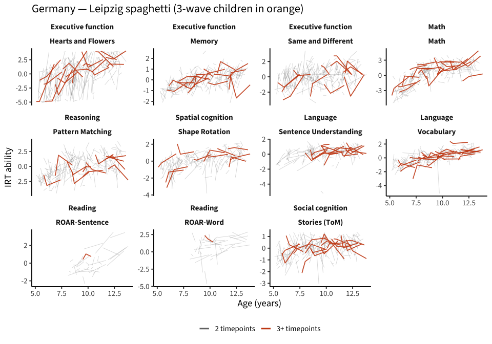
spaghetti("pilot_uniandes_co_bogota", "Colombia — Bogotá spaghetti")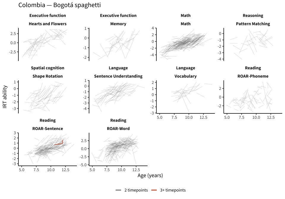
spaghetti("pilot_uniandes_co_rural",
          "Colombia — Caquetá/Boyacá spaghetti (new in 2026-08; sparse panels suppressed)")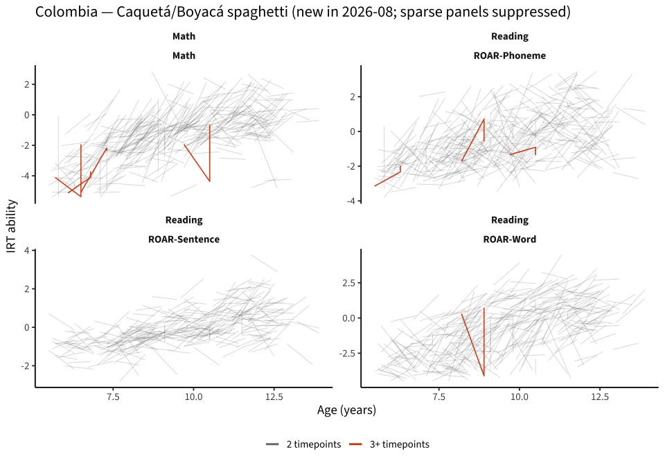
(Rural’s few ≥3-run children include short-gap repeat administrations — the near-vertical orange segments; treat those individual trajectories with care. Leipzig’s orange three-wave children, by contrast, are the designed third wave.)
spaghetti("pilot_western_ca_main", "Canada — Ontario spaghetti")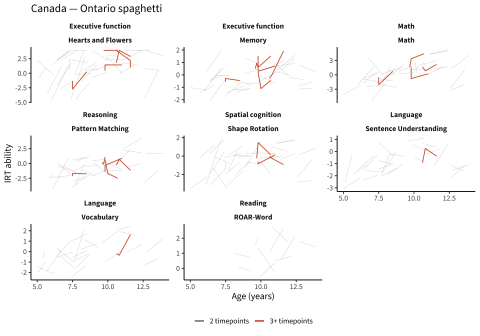
Simple growth models per (dataset, task)
For each (dataset, task), fit
score ~ age_c + (1 | user_id)
with age_c = age − mean(age). With mostly 2 timepoints the random-slope variance is unidentifiable, so we read the fixed effect of age_c as the average within-individual slope. Per-child heterogeneity is examined separately below.
Where both adaptive and non-adaptive versions are present we include adaptive as a fixed effect.
fit_growth <- function(df) {
  df <- df |> mutate(age_c = age - mean(age, na.rm = TRUE))
  has_both_adaptive <- length(unique(na.omit(df$adaptive))) > 1
  fm <- if (has_both_adaptive) {
    score ~ age_c + adaptive + (1 | user_id)
  } else {
    score ~ age_c + (1 | user_id)
  }
  tryCatch(
    lmer(fm, data = df, REML = TRUE,
         control = lmerControl(optimizer = "bobyqa",
                               optCtrl = list(maxfun = 2e5))),
    error = function(e) {
      message(glue("  fit failed: {conditionMessage(e)}"))
      NULL
    }
  )
}

growth_data <- scores |>
  group_by(dataset, task_id) |>
  filter(n_distinct(user_id[duplicated(user_id) | duplicated(user_id, fromLast = TRUE)]) >= 30) |>
  ungroup()

growth_fits <- growth_data |>
  group_by(dataset, dataset_label, task_id, task_label, task_category) |>
  nest() |>
  mutate(fit = map(data, fit_growth)) |>
  filter(!map_lgl(fit, is.null))

glue("Fitted {nrow(growth_fits)} (dataset, task) growth models.")
Fitted 28 (dataset, task) growth models.within_slopes <- growth_fits |>
mutate(coef_tbl = map(fit, \(m) broom.mixed::tidy(m, effects = "fixed",
conf.int = TRUE))) |>
select(dataset_label, task_label, task_category, coef_tbl) |>
unnest(coef_tbl) |>
filter(term == "age_c") |>
select(dataset_label, task_label, task_category,
within_slope = estimate, within_slope_se = std.error,
within_ci_lo = conf.low, within_ci_hi = conf.high)
knitr::kable(within_slopes, digits = 3)| dataset | task_id | dataset_label | task_label | task_category | within_slope | within_slope_se | within_ci_lo | within_ci_hi |
|---|---|---|---|---|---|---|---|---|
| pilot_mpieva_de_main | hearts-and-flowers | Germany — Leipzig | Hearts and Flowers | Executive function | 0.660 | 0.046 | 0.569 | 0.751 |
| pilot_mpieva_de_main | egma-math | Germany — Leipzig | Math | Math | 0.608 | 0.036 | 0.537 | 0.679 |
| pilot_mpieva_de_main | matrix-reasoning | Germany — Leipzig | Pattern Matching | Reasoning | 0.352 | 0.035 | 0.284 | 0.420 |
| pilot_mpieva_de_main | memory-game | Germany — Leipzig | Memory | Executive function | 0.197 | 0.015 | 0.167 | 0.226 |
| pilot_mpieva_de_main | mental-rotation | Germany — Leipzig | Shape Rotation | Spatial cognition | 0.217 | 0.021 | 0.176 | 0.258 |
| pilot_mpieva_de_main | same-different-selection | Germany — Leipzig | Same and Different | Executive function | 0.129 | 0.027 | 0.076 | 0.182 |
| pilot_mpieva_de_main | theory-of-mind | Germany — Leipzig | Stories (ToM) | Social cognition | 0.119 | 0.016 | 0.088 | 0.150 |
| pilot_mpieva_de_main | trog | Germany — Leipzig | Sentence Understanding | Language | 0.140 | 0.018 | 0.105 | 0.176 |
| pilot_mpieva_de_main | vocab | Germany — Leipzig | Vocabulary | Language | 0.260 | 0.016 | 0.230 | 0.290 |
| pilot_mpieva_de_main | sre | Germany — Leipzig | ROAR-Sentence | Reading | 0.364 | 0.037 | 0.292 | 0.437 |
| pilot_mpieva_de_main | swr | Germany — Leipzig | ROAR-Word | Reading | 0.311 | 0.060 | 0.194 | 0.428 |
| pilot_uniandes_co_bogota | hearts-and-flowers | Colombia — Bogotá | Hearts and Flowers | Executive function | 0.483 | 0.037 | 0.410 | 0.555 |
| pilot_uniandes_co_bogota | egma-math | Colombia — Bogotá | Math | Math | 0.561 | 0.023 | 0.515 | 0.606 |
| pilot_uniandes_co_bogota | memory-game | Colombia — Bogotá | Memory | Executive function | 0.260 | 0.023 | 0.215 | 0.305 |
| pilot_uniandes_co_bogota | sre | Colombia — Bogotá | ROAR-Sentence | Reading | 0.346 | 0.017 | 0.313 | 0.380 |
| pilot_uniandes_co_bogota | pa | Colombia — Bogotá | ROAR-Phoneme | Reading | 0.391 | 0.036 | 0.321 | 0.462 |
| pilot_uniandes_co_bogota | swr | Colombia — Bogotá | ROAR-Word | Reading | 0.560 | 0.031 | 0.500 | 0.621 |
| pilot_uniandes_co_bogota | trog | Colombia — Bogotá | Sentence Understanding | Language | 0.264 | 0.021 | 0.222 | 0.305 |
| pilot_uniandes_co_bogota | mental-rotation | Colombia — Bogotá | Shape Rotation | Spatial cognition | 0.345 | 0.028 | 0.291 | 0.399 |
| pilot_uniandes_co_rural | egma-math | Colombia — Caquetá/Boyacá | Math | Math | 0.472 | 0.022 | 0.428 | 0.516 |
| pilot_uniandes_co_rural | swr | Colombia — Caquetá/Boyacá | ROAR-Word | Reading | 0.511 | 0.028 | 0.455 | 0.566 |
| pilot_uniandes_co_rural | sre | Colombia — Caquetá/Boyacá | ROAR-Sentence | Reading | 0.236 | 0.016 | 0.206 | 0.267 |
| pilot_uniandes_co_rural | pa | Colombia — Caquetá/Boyacá | ROAR-Phoneme | Reading | 0.287 | 0.021 | 0.246 | 0.327 |
| pilot_western_ca_main | hearts-and-flowers | Canada — Ontario | Hearts and Flowers | Executive function | 0.349 | 0.048 | 0.254 | 0.443 |
| pilot_western_ca_main | egma-math | Canada — Ontario | Math | Math | 0.727 | 0.040 | 0.648 | 0.806 |
| pilot_western_ca_main | matrix-reasoning | Canada — Ontario | Pattern Matching | Reasoning | 0.430 | 0.036 | 0.360 | 0.500 |
| pilot_western_ca_main | memory-game | Canada — Ontario | Memory | Executive function | 0.270 | 0.021 | 0.229 | 0.311 |
| pilot_western_ca_main | mental-rotation | Canada — Ontario | Shape Rotation | Spatial cognition | 0.327 | 0.031 | 0.266 | 0.388 |
Cross-sectional age gradients for comparison
OLS slope of score on age within each (dataset, task), using each child’s first observation.
cross_slopes <- scores |>
  group_by(dataset, user_id, task_id) |>
  arrange(age) |>
  slice(1) |>
  ungroup() |>
  group_by(dataset, dataset_label, task_id, task_label, task_category) |>
  filter(n() >= 30) |>
  summarise(
    cross_slope = coef(lm(score ~ age))[2],
    cross_n     = n(),
    .groups = "drop"
  )

slope_compare <- within_slopes |>
  inner_join(cross_slopes, by = c("dataset_label", "task_label",
                                   "task_category"))

knitr::kable(slope_compare, digits = 3)| dataset.x | task_id.x | dataset_label | task_label | task_category | within_slope | within_slope_se | within_ci_lo | within_ci_hi | dataset.y | task_id.y | cross_slope | cross_n |
|---|---|---|---|---|---|---|---|---|---|---|---|---|
| pilot_mpieva_de_main | hearts-and-flowers | Germany — Leipzig | Hearts and Flowers | Executive function | 0.660 | 0.046 | 0.569 | 0.751 | pilot_mpieva_de_main | hearts-and-flowers | 0.699 | 337 |
| pilot_mpieva_de_main | egma-math | Germany — Leipzig | Math | Math | 0.608 | 0.036 | 0.537 | 0.679 | pilot_mpieva_de_main | egma-math | 0.665 | 310 |
| pilot_mpieva_de_main | matrix-reasoning | Germany — Leipzig | Pattern Matching | Reasoning | 0.352 | 0.035 | 0.284 | 0.420 | pilot_mpieva_de_main | matrix-reasoning | 0.411 | 310 |
| pilot_mpieva_de_main | memory-game | Germany — Leipzig | Memory | Executive function | 0.197 | 0.015 | 0.167 | 0.226 | pilot_mpieva_de_main | memory-game | 0.175 | 325 |
| pilot_mpieva_de_main | mental-rotation | Germany — Leipzig | Shape Rotation | Spatial cognition | 0.217 | 0.021 | 0.176 | 0.258 | pilot_mpieva_de_main | mental-rotation | 0.227 | 292 |
| pilot_mpieva_de_main | same-different-selection | Germany — Leipzig | Same and Different | Executive function | 0.129 | 0.027 | 0.076 | 0.182 | pilot_mpieva_de_main | same-different-selection | 0.128 | 331 |
| pilot_mpieva_de_main | theory-of-mind | Germany — Leipzig | Stories (ToM) | Social cognition | 0.119 | 0.016 | 0.088 | 0.150 | pilot_mpieva_de_main | theory-of-mind | 0.146 | 314 |
| pilot_mpieva_de_main | trog | Germany — Leipzig | Sentence Understanding | Language | 0.140 | 0.018 | 0.105 | 0.176 | pilot_mpieva_de_main | trog | 0.153 | 276 |
| pilot_mpieva_de_main | vocab | Germany — Leipzig | Vocabulary | Language | 0.260 | 0.016 | 0.230 | 0.290 | pilot_mpieva_de_main | vocab | 0.272 | 296 |
| pilot_mpieva_de_main | sre | Germany — Leipzig | ROAR-Sentence | Reading | 0.364 | 0.037 | 0.292 | 0.437 | pilot_mpieva_de_main | sre | 0.323 | 162 |
| pilot_mpieva_de_main | swr | Germany — Leipzig | ROAR-Word | Reading | 0.311 | 0.060 | 0.194 | 0.428 | pilot_mpieva_de_main | swr | 0.322 | 164 |
| pilot_uniandes_co_bogota | hearts-and-flowers | Colombia — Bogotá | Hearts and Flowers | Executive function | 0.483 | 0.037 | 0.410 | 0.555 | pilot_uniandes_co_bogota | hearts-and-flowers | 0.489 | 383 |
| pilot_uniandes_co_bogota | egma-math | Colombia — Bogotá | Math | Math | 0.561 | 0.023 | 0.515 | 0.606 | pilot_uniandes_co_bogota | egma-math | 0.532 | 621 |
| pilot_uniandes_co_bogota | memory-game | Colombia — Bogotá | Memory | Executive function | 0.260 | 0.023 | 0.215 | 0.305 | pilot_uniandes_co_bogota | memory-game | 0.252 | 312 |
| pilot_uniandes_co_bogota | sre | Colombia — Bogotá | ROAR-Sentence | Reading | 0.346 | 0.017 | 0.313 | 0.380 | pilot_uniandes_co_bogota | sre | 0.328 | 553 |
| pilot_uniandes_co_bogota | pa | Colombia — Bogotá | ROAR-Phoneme | Reading | 0.391 | 0.036 | 0.321 | 0.462 | pilot_uniandes_co_bogota | pa | 0.414 | 521 |
| pilot_uniandes_co_bogota | swr | Colombia — Bogotá | ROAR-Word | Reading | 0.560 | 0.031 | 0.500 | 0.621 | pilot_uniandes_co_bogota | swr | 0.590 | 570 |
| pilot_uniandes_co_bogota | trog | Colombia — Bogotá | Sentence Understanding | Language | 0.264 | 0.021 | 0.222 | 0.305 | pilot_uniandes_co_bogota | trog | 0.254 | 379 |
| pilot_uniandes_co_bogota | mental-rotation | Colombia — Bogotá | Shape Rotation | Spatial cognition | 0.345 | 0.028 | 0.291 | 0.399 | pilot_uniandes_co_bogota | mental-rotation | 0.338 | 360 |
| pilot_uniandes_co_rural | egma-math | Colombia — Caquetá/Boyacá | Math | Math | 0.472 | 0.022 | 0.428 | 0.516 | pilot_uniandes_co_rural | egma-math | 0.463 | 868 |
| pilot_uniandes_co_rural | swr | Colombia — Caquetá/Boyacá | ROAR-Word | Reading | 0.511 | 0.028 | 0.455 | 0.566 | pilot_uniandes_co_rural | swr | 0.477 | 703 |
| pilot_uniandes_co_rural | sre | Colombia — Caquetá/Boyacá | ROAR-Sentence | Reading | 0.236 | 0.016 | 0.206 | 0.267 | pilot_uniandes_co_rural | sre | 0.223 | 666 |
| pilot_uniandes_co_rural | pa | Colombia — Caquetá/Boyacá | ROAR-Phoneme | Reading | 0.287 | 0.021 | 0.246 | 0.327 | pilot_uniandes_co_rural | pa | 0.288 | 842 |
| pilot_western_ca_main | hearts-and-flowers | Canada — Ontario | Hearts and Flowers | Executive function | 0.349 | 0.048 | 0.254 | 0.443 | pilot_western_ca_main | hearts-and-flowers | 0.348 | 354 |
| pilot_western_ca_main | egma-math | Canada — Ontario | Math | Math | 0.727 | 0.040 | 0.648 | 0.806 | pilot_western_ca_main | egma-math | 0.721 | 333 |
| pilot_western_ca_main | matrix-reasoning | Canada — Ontario | Pattern Matching | Reasoning | 0.430 | 0.036 | 0.360 | 0.500 | pilot_western_ca_main | matrix-reasoning | 0.434 | 263 |
| pilot_western_ca_main | memory-game | Canada — Ontario | Memory | Executive function | 0.270 | 0.021 | 0.229 | 0.311 | pilot_western_ca_main | memory-game | 0.278 | 322 |
| pilot_western_ca_main | mental-rotation | Canada — Ontario | Shape Rotation | Spatial cognition | 0.327 | 0.031 | 0.266 | 0.388 | pilot_western_ca_main | mental-rotation | 0.333 | 308 |
slope_compare |>
  ggplot(aes(x = cross_slope, y = within_slope, color = task_category)) +
  geom_abline(slope = 1, intercept = 0, lty = 3, color = "grey50") +
  geom_hline(yintercept = 0, lty = 3, color = "grey80") +
  geom_vline(xintercept = 0, lty = 3, color = "grey80") +
  geom_errorbar(aes(ymin = within_ci_lo, ymax = within_ci_hi),
                alpha = 0.5, width = 0) +
  geom_point(size = 2.5) +
  geom_text_repel(aes(label = task_label), size = 3,
                  show.legend = FALSE, max.overlaps = 30) +
  facet_wrap(~dataset_label) +
  scale_colour_task() +
  labs(x = "Cross-sectional slope (per year)",
       y = "Within-child slope (per year)",
       title = "Within-child growth vs cross-sectional age gradient",
       subtitle = "Dotted line = identity",
       color = NULL) +
  theme(legend.position = "bottom")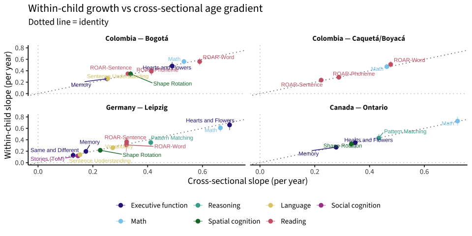
Fitted trajectories
Population-mean model curves overlaid on raw spaghetti, faceted by task.
predict_band <- function(fit, df) {
  if (is.null(fit)) return(NULL)
  age_grid <- seq(min(df$age, na.rm = TRUE),
                  max(df$age, na.rm = TRUE), length.out = 40)
  age_mean <- mean(df$age, na.rm = TRUE)
  newd <- tibble(age = age_grid, age_c = age_grid - age_mean)
  if ("adaptive" %in% all.vars(formula(fit))) newd$adaptive <- FALSE
  newd$score <- predict(fit, newdata = newd, re.form = NA,
                        allow.new.levels = TRUE)
  newd |> select(age, score)
}

fitted_lines <- growth_fits |>
  mutate(pred = map2(fit, data, predict_band)) |>
  select(dataset_label, task_label, task_category, pred) |>
  unnest(pred)

ggplot() +
  geom_line(data = repeats,
            aes(x = age, y = score, group = user_id),
            alpha = 0.15, color = "grey40") +
  geom_line(data = fitted_lines,
            aes(x = age, y = score, color = dataset_label),
            linewidth = 1) +
  facet_wrap(vars(task_category, task_label), scales = "free_y") +
  scale_color_brewer(palette = "Set1", name = NULL) +
  labs(title = "Fitted growth trajectories on top of raw spaghetti",
       x = "Age (years)", y = "IRT ability") +
  theme(legend.position = "bottom")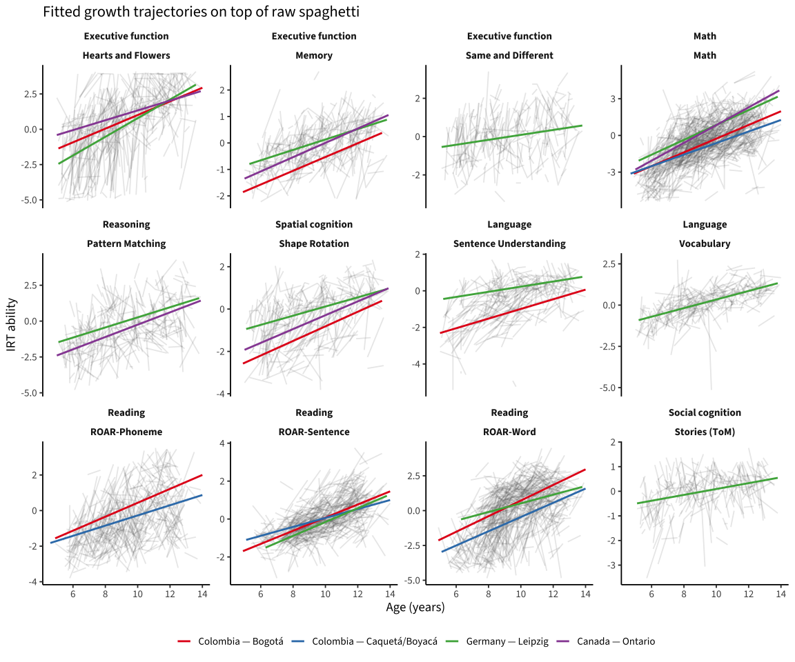
Child-level slopes
Per-child OLS slopes for kids with ≥ 2 runs (rise / run when N = 2).
child_slopes <- repeats |>
  group_by(dataset, dataset_label, task_id, task_label, task_category, user_id) |>
  filter(n_distinct(run_id) >= 2, diff(range(age)) > 0.1) |>
  summarise(
    n_runs    = n_distinct(run_id),
    age_mean  = mean(age),
    age_span  = diff(range(age)),
    slope     = coef(lm(score ~ age))[2],
    .groups = "drop"
  ) |>
  filter(is.finite(slope))

child_slopes |>
  group_by(dataset_label, task_label) |>
  filter(n() >= 30) |>
  ungroup() |>
  ggplot(aes(x = slope, fill = dataset_label)) +
  geom_histogram(bins = 30, alpha = 0.7, position = "identity") +
  geom_vline(xintercept = 0, lty = 3) +
  facet_wrap(vars(task_category, task_label), scales = "free") +
  scale_fill_brewer(palette = "Set1", name = NULL) +
  labs(title = "Per-child OLS slopes (per year)",
       x = "Slope of score on age",
       y = "Children") +
  theme(legend.position = "bottom")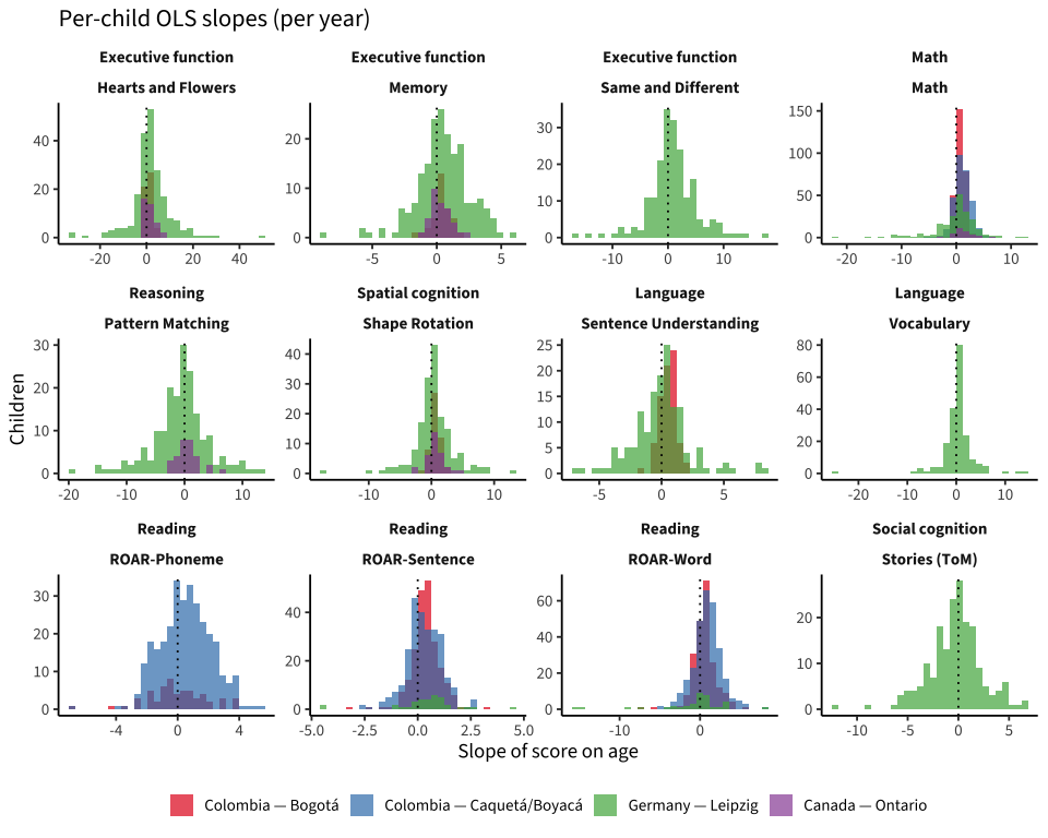
child_slopes |>
  group_by(dataset_label, task_label) |>
  summarise(n = n(), mean_slope = mean(slope), sd_slope = sd(slope),
            .groups = "drop") |>
  filter(n >= 30) |>
  arrange(dataset_label, task_label) |>
knitr::kable(digits = 3)| dataset_label | task_label | n | mean_slope | sd_slope |
|---|---|---|---|---|
| Colombia — Bogotá | Hearts and Flowers | 52 | 0.614 | 1.484 |
| Colombia — Bogotá | Math | 287 | 0.693 | 0.818 |
| Colombia — Bogotá | Memory | 32 | 0.371 | 0.724 |
| Colombia — Bogotá | ROAR-Phoneme | 56 | -0.078 | 1.994 |
| Colombia — Bogotá | ROAR-Sentence | 215 | 0.410 | 0.684 |
| Colombia — Bogotá | ROAR-Word | 216 | 0.489 | 1.457 |
| Colombia — Bogotá | Sentence Understanding | 75 | 0.494 | 0.650 |
| Colombia — Bogotá | Shape Rotation | 50 | 0.609 | 0.729 |
| Colombia — Caquetá/Boyacá | Math | 297 | 1.064 | 1.540 |
| Colombia — Caquetá/Boyacá | ROAR-Phoneme | 307 | 0.514 | 1.686 |
| Colombia — Caquetá/Boyacá | ROAR-Sentence | 263 | 0.301 | 0.836 |
| Colombia — Caquetá/Boyacá | ROAR-Word | 295 | 0.821 | 1.750 |
| Germany — Leipzig | Hearts and Flowers | 207 | 1.749 | 8.785 |
| Germany — Leipzig | Math | 201 | -0.217 | 4.071 |
| Germany — Leipzig | Memory | 194 | 0.491 | 2.037 |
| Germany — Leipzig | Pattern Matching | 182 | -0.809 | 4.932 |
| Germany — Leipzig | ROAR-Sentence | 34 | 0.438 | 1.632 |
| Germany — Leipzig | ROAR-Word | 37 | -0.996 | 4.505 |
| Germany — Leipzig | Same and Different | 196 | 0.825 | 4.389 |
| Germany — Leipzig | Sentence Understanding | 147 | -0.084 | 2.338 |
| Germany — Leipzig | Shape Rotation | 168 | 0.400 | 3.319 |
| Germany — Leipzig | Stories (ToM) | 187 | -0.328 | 2.626 |
| Germany — Leipzig | Vocabulary | 201 | 0.306 | 3.200 |
| Canada — Ontario | Hearts and Flowers | 38 | 1.281 | 2.301 |
| Canada — Ontario | Math | 31 | 1.309 | 1.773 |
| Canada — Ontario | Memory | 33 | 0.354 | 0.746 |
| Canada — Ontario | Pattern Matching | 30 | 0.594 | 2.003 |
| Canada — Ontario | Shape Rotation | 33 | 0.667 | 1.393 |
Save outputs
write_rds(within_slopes,  here("data", "growth_within_slopes.rds"))
write_rds(slope_compare,  here("data", "growth_slope_comparison.rds"))
write_rds(child_slopes,   here("data", "growth_child_slopes.rds"))

glue("Saved within-slope and per-child slope tables to data/.")
Saved within-slope and per-child slope tables to data/.Open questions for 02
- The CO-bog 1-year gap means most kids only have 2 timepoints. That’s enough to estimate a slope per child, but the per-individual SE is large. The latent-growth approach in 02 pools across tasks/constructs.
- mpieva-de’s 3- and 7-month gaps give a within-year change estimate that should be small in absolute terms; per-child OLS slopes there are noisy.
- Tasks with adaptive/non-adaptive mixing (vocab in mpieva-de especially) might bias estimates; flagged again in 02.