Hearts & Flowers v2 — feedback sound, faster mixed blocks: did it help?
ImportantAI-generated — not for publication
The code and prose in this chapter were written by Claude Code (an AI coding agent) under human direction. They have not been line-by-line verified by a human and must not be published or cited as-is.
WarningPreliminary & unvetted analysis
These are exploratory analyses of preliminary, in-progress LEVANTE data. Results have not been reviewed or validated and require checking by the LEVANTE Data Coordinating Center before any use.
Question
In spring 2026 Hearts & Flowers got a redesign (“version 2”). Two changes were intended: a feedback sound (“ding”) and a third mixed block run at different speeds. Did the revision help? Specifically: does the ding help or hurt, does the new form buy reliability, and does it remove the known ceiling? The two changes shipped together, so they are confounded by design; the strategy here is to find outcomes that only one of them should move.
Data: levante_data_latest:e9pf:v3_17 (scores, processed trials) plus the raw per-site trials/runs/variants tables (13 sites, pulled 2026-10-15 by _prep_hf_v2.R; derivations in _hf_v2_common.R).
The redesign is core-tasks PR #442 (merged 2026-04-21, first shipped in task version 1.1.2), gated on the variant parameter taskVersion === 2. That parameter isn’t exported to the Redivis variants table, but every variant created from 2026-04-23 on runs the new form, and every variant created 2025-07-21 (the legacy de / es-CO / English (North America) - Legacy variants) runs the old form, regardless of code version: old variants still produce the 32-trial mixed block on code 1.3.17.
Code
runs |>filter(layout !="incomplete") |>count(form, variant_name, variant_created =substr(variant_created, 1, 10), layout) |>pivot_wider(names_from = layout, values_from = n, values_fill =0) |>arrange(form, variant_created) |> knitr::kable(caption ="H&F variants by intended form (complete runs only; variant names repeat across site datasets)")
H&F variants by intended form (complete runs only; variant names repeat across site datasets)
form
variant_name
variant_created
v1 complete (32 mixed)
v2 complete (48 mixed)
v2 heavyInstructions (16 mixed)
v1
English (North America) - Legacy
2025-07-21
366
0
0
v1
de
2025-07-21
745
0
0
v1
es-CO
2025-07-21
789
0
0
v1
NA
2025-07-21
31
0
0
v2
English (North America)
2026-04-23
0
97
35
v2
es-AR
2026-04-23
0
915
0
v2
English (United Kingdom)
2026-07-31
0
226
2
v2
German (Germany)
2026-08-17
0
208
7
v2
Spanish (Colombia)
2026-08-17
0
328
4
What v2 changes, read from the code:
v1 (old)
v2 (new)
Response deadline
none (configured presentation times were dead code)
coin sound if correct, fail sound if not, every test trial
No response
impossible
response = null, scored incorrect
Early stop
effectively none (maxIncorrect = 100)
shared rule: stop if > 6 of the last 10 test trials are wrong
heavyInstructions variants
—
mixed block cut to the first 16 trials
Note that the early-stop rule’s code comment says “4 of the last 10” but the code tests > 6. Timeouts count as errors for it.
Scoring is unchanged across forms: the released multigroup_dataset Rasch model uses the same item uids (hf_{block}_{stim}_{start|stay|switch}) for both, and recode_hf() still marks every response faster than 200 ms or slower than 2000 ms incorrect. (I checked whether processing drops timeouts. It does not: all raw no-response trials are in the processed table, scored incorrect.)
2. Mechanics: the new segments make the task harder only through time
Code
mech <- hf_test |>semi_join(complete_runs, by ="run_id") |>filter(!is.na(block)) |>group_by(form, block, segment, window) |>summarise(trials =n(),correct_side_if_answered =mean(correct[!timeout] %in%TRUE),timeout =mean(timeout),rt_over_2s =mean(rt_numeric >2000, na.rm =TRUE),scored_correct =mean(sc_pipeline),median_rt =median(rt_numeric, na.rm =TRUE), .groups ="drop") |>mutate(block =factor(block, c("hearts", "flowers", "mixed"))) |>arrange(form, block, segment)knitr::kable(mech, digits =3,caption ="Trial-level mechanics, complete runs. window = response deadline (Inf = untimed v1). scored_correct = as released (timeouts and RT outside 200-2000 ms are errors).")
Trial-level mechanics, complete runs. window = response deadline (Inf = untimed v1). scored_correct = as released (timeouts and RT outside 200-2000 ms are errors).
form
block
segment
window
trials
correct_side_if_answered
timeout
rt_over_2s
scored_correct
median_rt
v1
hearts
NA
Inf
23172
0.974
0.000
0.059
0.910
769
v1
flowers
NA
Inf
30896
0.941
0.000
0.075
0.864
903
v1
mixed
1
Inf
30896
0.905
0.000
0.131
0.775
1182
v1
mixed
2
Inf
30896
0.911
0.000
0.154
0.757
1214
v2
hearts
NA
3000
21288
0.981
0.002
0.003
0.971
655
v2
flowers
NA
3000
28384
0.972
0.003
0.007
0.960
790
v2
mixed
1
3000
28384
0.919
0.006
0.025
0.890
1041
v2
mixed
2
2000
28384
0.914
0.029
0.000
0.886
974
v2
mixed
3
1500
28384
0.910
0.083
0.000
0.831
923
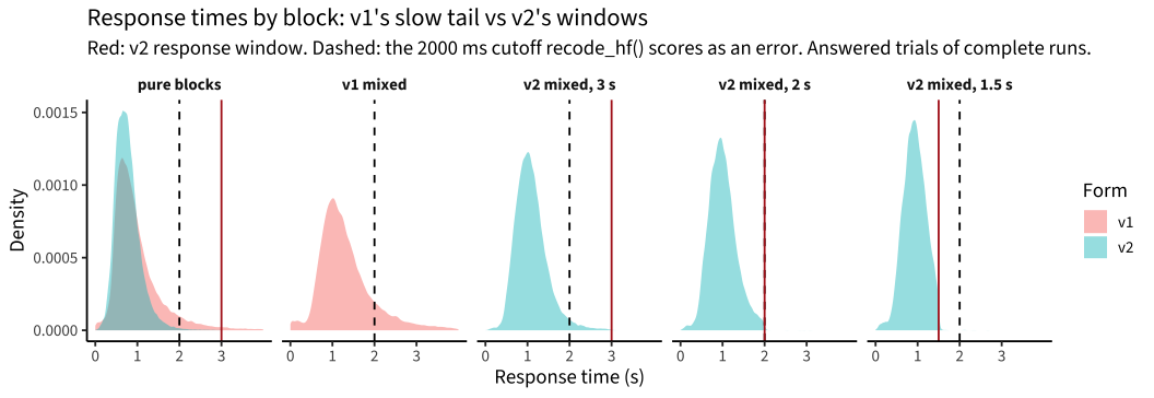
Within v2 the three mixed segments differ only in their deadline (the feedback is constant), so they isolate the timing manipulation. Shortening the window from 3 s to 2 s to 1.5 s raises timeouts from 0.6% to 2.9% to 8.3%, and that is most of the drop in scored accuracy (.89 → .83); the rest is a small decline in accuracy on answered trials. The faster segments add difficulty mainly by making children miss the window.
Across forms, the bigger effect is on slow responses. Untimed v1 children answered after 2 s on 6–15% of trials, all of which recode_hf() scores incorrect. Under v2’s deadlines and feedback that share falls to 0–2.5%. One mismatch follows: in the 3-s windows (pure blocks and mixed segment 1), a correct 2–3 s response plays the coin but is scored wrong (0.3–2.5% of those trials).
Code
rt_panels <- hf_test |>semi_join(complete_runs, by ="run_id") |>filter(!is.na(block), !timeout, rt_numeric >0, rt_numeric <4000) |>mutate(panel =case_when(block !="mixed"~"pure blocks", form =="v1"~"v1 mixed",TRUE~paste0("v2 mixed, ", window /1000, " s")),panel =factor(panel, c("pure blocks", "v1 mixed", "v2 mixed, 3 s","v2 mixed, 2 s", "v2 mixed, 1.5 s")))windows <-tibble(panel =factor(c("pure blocks", "v2 mixed, 3 s", "v2 mixed, 2 s","v2 mixed, 1.5 s"), levels(rt_panels$panel)),window =c(3000, 3000, 2000, 1500))ggplot(rt_panels, aes(rt_numeric, fill = form)) +geom_density(alpha = .45, colour =NA, adjust = .8) +geom_vline(xintercept =2000, linetype ="dashed") +geom_vline(data = windows, aes(xintercept = window), colour ="firebrick") +facet_wrap(~panel, nrow =1) +scale_x_continuous(breaks =c(0, 1000, 2000, 3000), labels =c("0", "1", "2", "3")) +labs(x ="Response time (s)", y ="Density", fill ="Form",title ="Response times by block: v1's slow tail vs v2's windows",subtitle ="Red: v2 response window. Dashed: the 2000 ms cutoff recode_hf() scores as an error. Answered trials of complete runs.")
The untimed v1 distributions have a long right tail past 2 s, all of which is scored as error. v2’s windows cut the tail off, and in the 2-s and 1.5-s segments the whole distribution shifts left as children speed up.
3. Many more v2 runs end early
Code
runs |>filter(!grepl("heavy", layout)) |>group_by(dataset) |>filter(n_distinct(form) ==2) |>ungroup() |>group_by(form) |>summarise(runs =n(), incomplete =mean(layout =="incomplete"), .groups ="drop") |> knitr::kable(digits =3, caption ="Share of runs that end before the last trial, sites that ran both forms")
Share of runs that end before the last trial, sites that ran both forms
Where incomplete runs stop (block and mixed segment)
where_stopped
v1
v2
flowers
32
83
hearts
25
28
mixed 1
13
99
mixed 2
29
141
mixed 3
0
230
Code
runs |>filter(form =="v2", layout =="incomplete") |>count(stop_reason) |> knitr::kable(caption ="stop_reason for incomplete v2 runs (logged from 2026-07-31 only)")
stop_reason for incomplete v2 runs (logged from 2026-07-31 only)
stop_reason
n
errorOut
293
sufficientTrials
6
taskAbort
14
timeOut
30
NA
238
About a quarter of v2 runs stop early (29% at sites that ran both forms), against 5% of v1 runs. Most v2 stops (371 of 581) fall in the 2-s and 1.5-s segments, and 293 of the 343 stops with a logged reason are errorOut. That is the rule working as written: timeouts count as errors, so a child who can’t keep up with the 1.5-s pace is stopped. The truncation is response-dependent, so θ estimates from the observed trials stay valid, but these children lose their hardest trials and many leave the task on a run of failures.
4. Floor and ceiling: the floor nearly disappears, the ceiling moves
Code
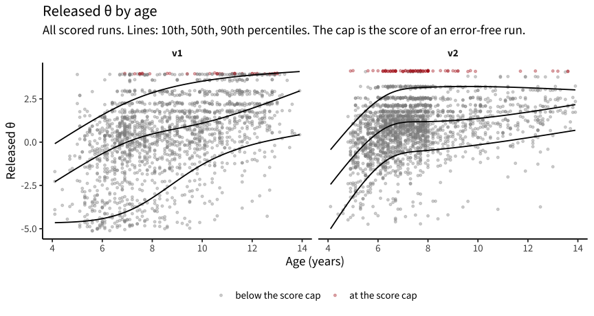
theta_age <- scored_runs |>filter(!is.na(age), age >=4, age <14) |>group_by(form) |>mutate(at_cap = theta >=max(theta) -0.05) |>ungroup()ggplot(theta_age, aes(age, theta)) +geom_point(aes(colour = at_cap), alpha =0.35, size =0.9) +geom_quantile(quantiles =c(.1, .5, .9), formula = y ~ splines::ns(x, 3),colour ="black") +facet_wrap(~form) +scale_colour_manual(values =c(`FALSE`="grey55", `TRUE`="firebrick"),labels =c("below the score cap", "at the score cap"), name =NULL) +labs(x ="Age (years)", y ="Released θ",title ="Released θ by age",subtitle ="All scored runs. Lines: 10th, 50th, 90th percentiles. The cap is the score of an error-free run.") +theme(legend.position ="bottom")
Code
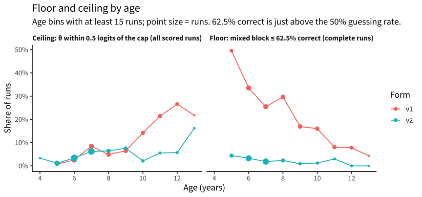
run_acc <- hf_test |>semi_join(complete_runs, by ="run_id") |>filter(!is.na(block)) |>group_by(run_id) |>summarise(acc =mean(sc_pipeline),acc_mixed =mean(sc_pipeline[block =="mixed"]),perfect_mixed =all(sc_pipeline[block =="mixed"]), .groups ="drop")ceiling_share <- scored_runs |>filter(!is.na(age), age >=4, age <14) |>group_by(form) |>mutate(near_cap = theta >=max(theta) -0.5) |>group_by(form, age_yr =floor(age)) |>summarise(n =n(), share =mean(near_cap), .groups ="drop") |>mutate(end ="Ceiling: θ within 0.5 logits of the cap (all scored runs)")floor_share <- complete_runs |>inner_join(run_acc, by ="run_id") |>filter(!is.na(age), age >=4, age <14) |>group_by(form, age_yr =floor(age)) |>summarise(n =n(), share =mean(acc_mixed <= .625), .groups ="drop") |>mutate(end ="Floor: mixed block ≤ 62.5% correct (complete runs)")bind_rows(ceiling_share, floor_share) |>filter(n >=15) |>ggplot(aes(age_yr, share, colour = form)) +geom_line() +geom_point(aes(size = n)) +facet_wrap(~end) +scale_size_area(max_size =4, guide ="none") +scale_y_continuous(labels = scales::percent) +scale_x_continuous(breaks =seq(4, 13, 2)) +labs(x ="Age (years)", y ="Share of runs", colour ="Form",title ="Floor and ceiling by age",subtitle ="Age bins with at least 15 runs; point size = runs. 62.5% correct is just above the 50% guessing rate.")
Code
complete_runs |>inner_join(run_acc, by ="run_id") |>filter(!is.na(age)) |>group_by(form, age =age_band(age)) |>summarise(runs =n(), mean_scored_acc =mean(acc),perfect_mixed =mean(perfect_mixed),acc_97_plus =mean(acc >= .97), .groups ="drop") |>pivot_wider(names_from = form, values_from =-c(form, age)) |> knitr::kable(digits =3, caption ="Accuracy-based ceiling indicators by age band, complete runs. Note the mixed block is 32 trials in v1 and 48 in v2, so a perfect mixed block is harder to achieve in v2 regardless of difficulty.")
Accuracy-based ceiling indicators by age band, complete runs. Note the mixed block is 32 trials in v1 and 48 in v2, so a perfect mixed block is harder to achieve in v2 regardless of difficulty.
age
runs_v1
runs_v2
mean_scored_acc_v1
mean_scored_acc_v2
perfect_mixed_v1
perfect_mixed_v2
acc_97_plus_v1
acc_97_plus_v2
<6
146
189
0.656
0.863
0.007
0.032
0.027
0.069
6-8
623
1028
0.773
0.903
0.074
0.055
0.093
0.191
8-10
482
281
0.823
0.910
0.079
0.082
0.139
0.224
10+
574
276
0.909
0.930
0.220
0.083
0.331
0.286
Code
scored_runs |>filter(!is.na(age)) |>group_by(form) |>mutate(cap =max(theta)) |>group_by(form, age =age_band5(age)) |>summarise(runs =n(), at_cap =mean(theta >= cap -0.05),within_half_logit =mean(theta >= cap -0.5), .groups ="drop") |>pivot_wider(names_from = form, values_from =-c(form, age)) |> knitr::kable(digits =3, caption ="θ-scale ceiling by age band, all scored runs (cap = 4.0 in v1, 4.13 in v2)")
θ-scale ceiling by age band, all scored runs (cap = 4.0 in v1, 4.13 in v2)
age
runs_v1
runs_v2
at_cap_v1
at_cap_v2
within_half_logit_v1
within_half_logit_v2
<6
156
412
0.000
0.010
0.006
0.012
6-8
622
1274
0.011
0.044
0.055
0.048
8-10
476
320
0.008
0.062
0.057
0.069
10-12
400
166
0.028
0.006
0.178
0.036
12+
169
131
0.083
0.053
0.260
0.092
The floor nearly disappears. In v1, half of 5-year-olds and a third of 6-year-olds scored near chance on the mixed block, as did 17–30% of 7- to 9-year-olds. In v2 that share is under 5% at every age. Part of v1’s floor was slow responding: answers after 2 s are scored as errors (§2), and v1 children gave many of them.
The ceiling can’t be judged on released θ. The released model scores v2 with item parameters calibrated on untimed v1 trials, so passing a 1.5-s switch trial earns the same credit as an untimed pass, and the top of the v2 distribution is capped by items that are too easy for it. On released θ the picture is mixed: fewer of the oldest children sit within half a logit of the cap in v2 (10–12: 18% vs 4%; 12+: 26% vs 9%), but more 6- to 10-year-olds sit exactly at it (4–6% vs about 1%). §11 refits both forms on one scale, with the timed items calibrated separately, and that is the comparison to use: v2 does reduce the ceiling substantially.
The accuracy indicators in the table are confounded too: the v2 mixed block is half again as long (48 vs 32 trials), so a perfect block is harder to achieve whatever the items’ difficulty. (An earlier version of this section read that as the fast segment cutting the ceiling.)
On raw split-half, v1 looks more reliable (.96 vs .86). Part of that is a stable individual difference v2 suppresses on purpose: in untimed v1, a child’s share of responses slower than 2 s is almost perfectly consistent (.95), and those responses are scored as errors. Under v2’s deadlines that trait is much less reliable (.68). v1 still leads on side-correctness alone (.93 vs .83).
Model-based reliability of θ (all scored runs)
Code
scored_runs |>group_by(form, dataset) |>filter(n() >=30) |>summarise(runs =n(), incomplete =mean(layout =="incomplete"),sd_theta =sd(theta), mean_se =mean(theta_se),reliability =var(theta) / (var(theta) +mean(theta_se^2)),.groups ="drop") |> knitr::kable(digits =3, caption ="Empirical reliability of released θ by dataset and form, all scored runs (incomplete runs included)")
Empirical reliability of released θ by dataset and form, all scored runs (incomplete runs included)
form
dataset
runs
incomplete
sd_theta
mean_se
reliability
v1
partner_mpib_de_main
209
0.000
1.658
0.645
0.861
v1
pilot_mpieva_de_main
545
0.039
2.647
0.726
0.926
v1
pilot_uniandes_co_bogota
519
0.042
1.902
0.639
0.893
v1
pilot_uniandes_co_rural
270
0.011
1.990
0.635
0.903
v1
pilot_western_ca_main
348
0.017
2.259
0.724
0.901
v1
rfp1_utdt_intl_ys
30
0.033
2.178
0.695
0.902
v2
pilot_bostonchildrens_us_main
61
0.721
2.434
0.765
0.904
v2
pilot_capecoast_gh_main
42
0.690
2.237
0.689
0.907
v2
pilot_mpieva_de_main
202
0.069
1.092
0.645
0.729
v2
pilot_uniandes_co_bogota
100
0.100
1.596
0.596
0.870
v2
pilot_uniandes_co_rural
230
0.261
1.542
0.557
0.879
v2
pilot_western_ca_main
87
0.241
1.748
0.590
0.892
v2
rfp1_sheffield_gb_main
269
0.164
1.449
0.589
0.849
v2
rfp1_utdt_ar_main
947
0.156
1.467
0.599
0.848
v2
rfp1_utdt_intl_ys
331
0.462
1.559
0.583
0.869
Counting every scored run (including the children stopped early), v2’s model-based reliability is .85–.91 at most sites, about the same as v1’s .86–.93. Leipzig’s wave 3 is the exception (.73): those children are older, and their v2 scores are compressed (SD 1.1 vs 2.6 for v1). Restricting to complete runs would understate v2 (it drops its weakest children), so these all-runs numbers are the fair comparison. The new form does not add reliability; at best it holds it.
Retest correlation of θ by form pair (consecutive runs, >= 14 days apart, n >= 10)
dataset
forms
pairs
median_gap_days
age_t2
sd_theta_t2
r
partner_mpib_de_main
v1 -> v2
14
228.53
7.46
1.25
-0.63
pilot_bostonchildrens_us_main
v2 -> v2
11
20.99
4.47
2.30
0.93
pilot_mpieva_de_main
v1 -> v1
209
111.82
9.18
2.50
0.54
pilot_mpieva_de_main
v1 -> v2
197
490.07
10.57
1.08
0.12
pilot_uniandes_co_bogota
v1 -> v1
64
490.04
9.47
1.48
0.49
pilot_uniandes_co_bogota
v1 -> v2
17
868.19
10.36
1.19
0.34
pilot_western_ca_main
v1 -> v1
37
394.99
10.14
1.58
0.58
pilot_western_ca_main
v1 -> v2
11
363.03
8.62
1.79
0.55
The only large cross-form sample is Leipzig: wave 1 → wave 2 (both v1) retests at .54, while wave 2 (v1) → wave 3 (v2) retests at .12. Three things are confounded in that drop: the form change, a much longer gap (~16 vs ~4 months), and range restriction in the older wave-3 sample (θ SD 1.1). Bogotá’s 17 cross-form pairs (~28 months apart) retest at .34, against .49 for its 64 v1 → v1 pairs (~16 months). Western’s small cross-form sample (n = 11, ~1 year) retests about like its v1 → v1 pairs (.55 vs .58), while MPIB’s 14 cross-form pairs (~7.5 months, age ~7.5) come out negative (−.63). There is no adequate v2 → v2 retest yet (Boston’s 11 pairs are three weeks apart, in 4-year-olds). Cross-form continuity is not established, and the Leipzig number is a warning for any longitudinal analysis that spans the switch.
6. Age validity
Code
scored_runs |>filter(!is.na(age)) |>group_by(dataset) |>filter(n_distinct(form) ==2) |>group_by(dataset, form) |>filter(n() >=30) |>summarise(runs =n(), mean_age =mean(age), sd_age =sd(age),r_theta_age =cor(theta, age),logits_per_year =coef(lm(theta ~ age))[2], .groups ="drop") |> knitr::kable(digits =2, caption ="θ–age association within sites that ran both forms, all scored runs")
θ–age association within sites that ran both forms, all scored runs
dataset
form
runs
mean_age
sd_age
r_theta_age
logits_per_year
partner_mpib_de_main
v1
209
7.12
0.62
0.27
0.73
pilot_mpieva_de_main
v1
545
9.05
2.22
0.55
0.65
pilot_mpieva_de_main
v2
202
10.58
2.31
0.20
0.10
pilot_uniandes_co_bogota
v1
401
9.11
2.03
0.60
0.54
pilot_uniandes_co_bogota
v2
100
9.99
2.25
0.25
0.18
pilot_uniandes_co_rural
v1
270
9.23
2.25
0.41
0.36
pilot_uniandes_co_rural
v2
230
9.44
2.30
0.54
0.36
pilot_western_ca_main
v1
348
8.91
2.22
0.36
0.37
pilot_western_ca_main
v2
87
7.71
2.13
0.25
0.21
rfp1_utdt_intl_ys
v1
30
5.72
0.34
0.01
0.08
rfp1_utdt_intl_ys
v2
331
5.50
0.39
0.23
0.91
Age associations are weaker under v2 at most sites that ran both forms (the exception is rural Colombia). Sample age ranges differ by wave and site, so this is suggestive rather than decisive. It fits the compression seen above: v2 lifts the low end, so younger children look more like older ones.
7. The ding: a clean feedback signature
Feedback should change what happens after an error. The pure blocks are the best place to look, because the 3-s deadline almost never binds there (<1% timeouts) and only the feedback differs.
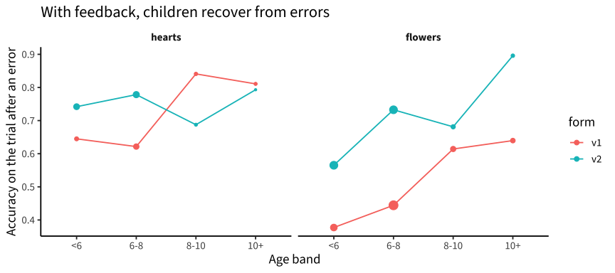
post_error |>filter(block !="mixed") |>ggplot(aes(x = age, y = acc_after_error, colour = form, group = form)) +geom_line() +geom_point(aes(size = error_trials)) +facet_wrap(~block) +scale_size_area(max_size =4, guide ="none") +labs(x ="Age band", y ="Accuracy on the trial after an error",title ="With feedback, children recover from errors")
Without feedback (v1), children speed up after an error (negative post-error slowing) and are often wrong again: post-error accuracy in the flowers block is .38–.64, a signature of being stuck on the wrong rule. With the coin/fail sound (v2), post-error slowing turns positive or near zero, and post-error accuracy rises sharply in every flowers age band (ages 6–8: .44 → .73; 10+: .64 → .90) and in the two younger hearts bands. In the hearts block from age 8, where errors are rare (29–88 per cell), it is slightly lower in v2. Accuracy after a correct trial is the same in both forms, so this isn’t a difference in the samples’ baseline ability.
So the ding does what feedback should: it breaks perseverative error runs. Whether that “helps” depends on what the task should measure. v1’s lower range was partly children who never grasped or held the flower rule; v2 corrects them within a few trials, which makes it more a measure of conflict efficiency and less of rule acquisition. That shift accounts for much of the low-end compression in sections 4–6.
8. Separating the two interventions
Outcome
Moved by
Evidence
Post-error recovery, pure blocks
feedback
v1 → v2 at matched post-correct accuracy (§7)
Timeouts, early stops in mixed
timing
dose-response across v2’s three segments, feedback constant (§2, §3)
Fewer slow (>2 s) responses
both
deadline caps them; feedback also speeds responses in the pure blocks, where the deadline barely binds
Fewer near-cap scores at 10+
timing (likely)
the 1.5-s segment is the only part of v2 that is hard for older children (§2, §9)
Higher scored accuracy at young ages
both, mostly feedback + fewer slow errors
§4, §7
Reliability, retest, age validity
not separable
only overall v1 vs v2 contrasts exist
9. Timing, calibration, and the ceiling
The redesign’s goal was to remove the ceiling and make the task harder for older children while measuring the same constructs. This section asks how well the timings serve that goal: where items of each timing sit relative to children’s abilities at each age, and whether shorter windows add information about inhibition and switching or about something else.
Where the released items sit
The released model is a Rasch model with a fixed guessing floor of 0.5, calibrated on 1,671 runs (registry v2_3, August 2026), essentially all of them untimed v1.
# "top decile" below = 90th percentile of v1 children aged 10 and overtop_decile <-unname(quantile(scored_runs$theta[scored_runs$form =="v1"& scored_runs$age >=10], .9, na.rm =TRUE))
The hardest released item (a mixed-block switch trial) sits at about +0.6, while median ability is above 1.7 from age 10 on and the top decile of children aged 10 and over sits near 3.9, close to the highest score the model gives. With a 0.5 guessing floor an item is most informative about half a logit above its difficulty, and its information can never exceed 0.09 per trial (a 2AFC item carries at most a quarter of the information of an item with no guessing floor).
Code
info_3pl <- \(theta, b, g =0.5) { p <- g + (1- g) *plogis(theta - b) ((p - g) / (1- g))^2* (1- p) / p}b_of <- \(uid) released$b[released$item_uid == uid]at <- theta_by_age |>select(age, theta = median) |>bind_rows(tibble(age ="top decile, ages 10+", theta = top_decile))info_tab <- released |>select(item_uid, b)for (i inseq_len(nrow(at))) info_tab[[at$age[i]]] <-info_3pl(at$theta[i], info_tab$b)knitr::kable(info_tab, digits =3, caption =sprintf("Fisher information per trial of each released item at the median θ of each age band and at the top decile of children 10+ (θ = %.1f); maximum possible 0.09", top_decile))
Fisher information per trial of each released item at the median θ of each age band and at the top decile of children 10+ (θ = 3.9); maximum possible 0.09
item_uid
b
<6
6-8
8-10
10-12
12+
top decile, ages 10+
hf_hearts_heart_start
-2.26
0.088
0.037
0.025
0.009
0.006
0.001
hf_hearts_heart_stay
-2.17
0.089
0.040
0.027
0.010
0.006
0.001
hf_flowers_flower_stay
-1.45
0.082
0.065
0.048
0.019
0.012
0.002
hf_flowers_flower_start
-1.22
0.074
0.073
0.056
0.023
0.015
0.003
hf_heartsflowers_flower_start
-0.46
0.041
0.090
0.082
0.043
0.030
0.006
hf_heartsflowers_flower_stay
-0.38
0.037
0.090
0.084
0.045
0.032
0.007
hf_heartsflowers_heart_stay
-0.30
0.034
0.090
0.085
0.048
0.034
0.007
hf_heartsflowers_flower_switch
0.20
0.018
0.080
0.090
0.066
0.049
0.012
hf_heartsflowers_heart_switch
0.50
0.011
0.069
0.086
0.076
0.060
0.015
hf_heartsflowers_heart_start
0.64
0.009
0.063
0.082
0.081
0.065
0.017
At the median 10- to 12-year-old, mixed-block switch trials are still fairly informative (about three-quarters of the maximum). The pure-block heart trials carry little information from age 8 (under a third of the maximum) and the flower trials from age 10 (about a quarter), and every untimed item gives at most a fifth of the maximum in the top decile. That top decile is the ceiling.
Deadline items on the released scale
v1 was untimed, so any deadline D can be imposed after the fact: score a response correct only if it is on the right side and 200 ms ≤ RT ≤ D, then estimate each released item’s difficulty with the children’s released θ held fixed. This puts every hypothetical deadline on the released scale (_hf_v2_deadlines.R).
Code
dl_file <-here("data/hf_v2/deadline_items.rds")if (!file.exists(dl_file)) source(here("tasks/_hf_v2_deadlines.R"))dl <-readRDS(dl_file)item_order <-c("hearts_heart_start", "hearts_heart_stay", "flowers_flower_start","flowers_flower_stay", "heartsflowers_heart_start", "heartsflowers_flower_start","heartsflowers_heart_stay", "heartsflowers_flower_stay","heartsflowers_heart_switch", "heartsflowers_flower_switch")dl$v1_items |>mutate(b =if_else(b >7.9, NA_real_, b),deadline =if_else(is.finite(deadline), paste0(deadline, " ms"), "untimed"),item =factor(paste0("hf_", item_class), paste0("hf_", item_order))) |>select(item, deadline, b) |>pivot_wider(names_from = deadline, values_from = b) |>arrange(item) |> knitr::kable(digits =2, caption ="Difficulty of each released item (released scale) when a deadline D is imposed on untimed v1 responses. Blank = accuracy below the 0.5 guessing floor, which the model cannot fit.")
Difficulty of each released item (released scale) when a deadline D is imposed on untimed v1 responses. Blank = accuracy below the 0.5 guessing floor, which the model cannot fit.
item
untimed
3000 ms
2500 ms
2000 ms
1750 ms
1500 ms
1250 ms
1000 ms
800 ms
hf_hearts_heart_start
-6.07
-3.58
-3.11
-2.13
-1.54
-0.65
0.44
1.83
5.15
hf_hearts_heart_stay
-3.92
-3.14
-2.80
-2.21
-1.72
-1.06
-0.17
1.37
4.09
hf_flowers_flower_start
-2.45
-1.87
-1.53
-1.09
-0.75
-0.09
1.00
2.89
NA
hf_flowers_flower_stay
-2.72
-2.24
-1.97
-1.43
-0.95
-0.26
0.84
2.93
NA
hf_heartsflowers_heart_start
-0.18
0.03
0.24
0.70
1.21
2.21
3.67
NA
NA
hf_heartsflowers_flower_start
-2.04
-1.41
-1.16
-0.48
0.03
1.13
2.53
6.70
NA
hf_heartsflowers_heart_stay
-1.99
-1.40
-1.02
-0.34
0.26
1.16
2.67
6.31
NA
hf_heartsflowers_flower_stay
-2.32
-1.59
-1.18
-0.36
0.30
1.40
3.15
NA
NA
hf_heartsflowers_heart_switch
-0.78
-0.39
-0.13
0.45
0.99
1.95
3.78
NA
NA
hf_heartsflowers_flower_switch
-1.32
-0.74
-0.45
0.18
0.80
1.88
3.87
NA
NA
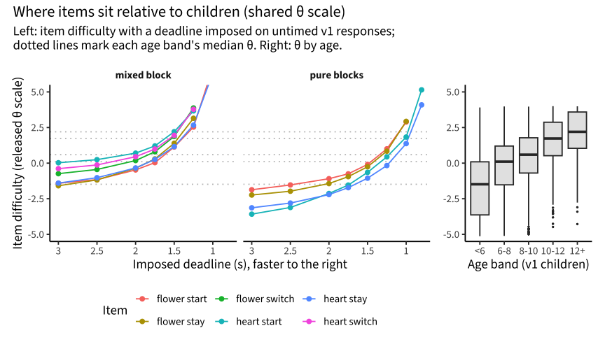
At D = 2000 ms (the cutoff recode_hf() applies today) the counterfactual difficulties reproduce the released ones, within 0.13 logits for every item. Tightening to 1500 ms moves the mixed items to about b = 1.1–2.2, right at the older children’s median ability; 1250 ms moves them to about 2.5–3.9, the top decile. Below about 1250 ms accuracy falls under 50%. A model with a 0.5 guessing floor cannot represent that: a child who misses the window scores 0, not chance.
Code
item_lines <- dl$v1_items |>filter(is.finite(deadline), b <7.9) |>mutate(block =if_else(grepl("^heartsflowers", item_class), "mixed block", "pure blocks"),item =sub("^(heartsflowers|hearts|flowers)_", "", item_class),item =sub("_", " ", item))p_items <-ggplot(item_lines, aes(deadline, b, colour = item)) +geom_hline(yintercept = theta_by_age$median, colour ="grey75", linetype ="dotted") +geom_line() +geom_point() +scale_x_reverse(breaks =c(3000, 2500, 2000, 1500, 1000),labels =c("3", "2.5", "2", "1.5", "1")) +coord_cartesian(ylim =c(-5, 5)) +facet_wrap(~block) +labs(x ="Imposed deadline (s), faster to the right", y ="Item difficulty (released θ scale)",colour ="Item") +theme(legend.position ="bottom") +guides(colour =guide_legend(nrow =2))p_people <- scored_runs |>filter(form =="v1", !is.na(age)) |>mutate(age =age_band5(age)) |>ggplot(aes(age, theta)) +geom_boxplot(outlier.size =0.5, fill ="grey90") +coord_cartesian(ylim =c(-5, 5)) +labs(x ="Age band (v1 children)", y =NULL)patchwork::wrap_plots(p_items, p_people, widths =c(3, 1)) + patchwork::plot_annotation(title ="Where items sit relative to children (shared θ scale)",subtitle ="Left: item difficulty with a deadline imposed on untimed v1 responses;\ndotted lines mark each age band's median θ. Right: θ by age.")
Read across: at a 3-s deadline (left) every item sits below the median child aged 6 and over, and the mixed-block items only rise into the 10–12 and 12+ range at about 1.5 s or faster.
The counterfactual can be checked against v2, where children really were given these windows. Imposing 2000 and 1500 ms on the v2 3-s segment predicts what the same children did in the 2-s and 1.5-s segments:
Code
dl$validation |>summarise(across(everything(), \(x) x[!is.na(x)][1])) |> knitr::kable(digits =3, caption ="Counterfactual vs actual accuracy, v2 runs with all three mixed segments")
Counterfactual vs actual accuracy, v2 runs with all three mixed segments
seg1_untruncated
imposed_2000
imposed_1500
actual_seg2
actual_seg3
0.907
0.877
0.77
0.875
0.801
It matches closely at 2000 ms (.877 vs .875) and slightly underestimates at 1500 ms (.770 vs .801): children speed up a little when the deadline is real, so the counterfactual is conservative.
Counterfactual accuracy on mixed-block switch trials (heart and flower together) by age and imposed deadline (v1 children)
age
D = Inf
D = 2000
D = 1750
D = 1500
D = 1250
D = 1000
<6
0.80
0.56
0.48
0.35
0.20
0.09
6-8
0.87
0.69
0.63
0.51
0.32
0.13
8-10
0.90
0.74
0.67
0.57
0.43
0.22
10-12
0.91
0.84
0.80
0.72
0.57
0.36
12+
0.92
0.88
0.84
0.77
0.64
0.42
Code
typed |>filter(form =="v2", !is.na(age), block =="mixed", type =="switch") |>group_by(age =age_band5(age), window) |>summarise(accuracy =mean(correct %in%TRUE&!timeout), .groups ="drop") |>pivot_wider(names_from = window, values_from = accuracy, names_prefix ="window ") |> knitr::kable(digits =2, caption ="Actual accuracy on mixed-block switch trials (heart and flower together) by age and window (v2 children)")
Actual accuracy on mixed-block switch trials (heart and flower together) by age and window (v2 children)
age
window 1500
window 2000
window 3000
<6
0.63
0.79
0.80
6-8
0.78
0.83
0.87
8-10
0.81
0.83
0.86
10-12
0.83
0.87
0.87
12+
0.88
0.90
0.91
In real data the 1.5-s window puts 10–12-year-olds at 83% correct on switch trials, close to the accuracy at which a 2AFC item with a 0.5 floor is most informative (about 81%). So that window is well targeted for the median older child. The 12+ group (88%) and the top decile need something faster: near 1.25 s in the counterfactual.
Do shorter windows still measure inhibition and switching?
If a deadline makes items harder on construct, the deadline score should keep tracking children’s switching skill (their untimed mixed-block accuracy), and the switch-vs-stay contrast should grow. If it only adds speed, the score should track plain response speed instead, measured here by the median RT on the easy same-side hearts trials.
Actual (v2): stay vs switch accuracy by stimulus and window
window
stimulus
stay
switch
switch_cost
3000
flower
0.927
0.864
0.064
2000
flower
0.881
0.837
0.044
1500
flower
0.824
0.771
0.053
3000
heart
0.922
0.848
0.074
2000
heart
0.904
0.831
0.073
1500
heart
0.862
0.780
0.082
In the counterfactual, the deadline score’s link to switching skill collapses as the window shortens (.49 at 2000 ms, .20 at 1500, .03 at 1250) while its link to plain speed stays around −.5 to −.6: a short fixed deadline turns the mixed block into a speed test. Real deadlines change behaviour, so the v2 data are the stronger test, and they point the same way by a different route: the switch cost barely changes as the window tightens (flower trials .064 at 3 s, .044 at 2 s, .053 at 1.5 s; heart trials .074, .073, .082). The deadline adds about the same difficulty to stay and switch trials rather than sharpening the inhibition and switching contrast.
rt_halves <- typed |>filter(form =="v1", block =="mixed", correct %in%TRUE) |>arrange(run_id, trial_index) |>group_by(run_id) |>mutate(half =row_number() %%2) |>group_by(run_id, half) |>summarise(switch_cost =median(rt_numeric[type =="switch"]) -median(rt_numeric[type =="stay"]),mixed_rt =median(rt_numeric), .groups ="drop")sb_halves <- \(v) { h <- rt_halves |>select(run_id, half, x =all_of(v)) |>pivot_wider(names_from = half, values_from = x) r <-cor(h$`0`, h$`1`, use ="complete.obs")2* r / (1+ r)}tibble(measure =c("RT switch cost (switch − stay median RT)", "mixed-block median RT"),split_half =c(sb_halves("switch_cost"), sb_halves("mixed_rt"))) |> knitr::kable(digits =2, caption ="Split-half reliability of RT measures, untimed v1 mixed block")
Split-half reliability of RT measures, untimed v1 mixed block
measure
split_half
RT switch cost (switch − stay median RT)
0.09
mixed-block median RT
0.95
A window scaled to each child’s own hearts-block speed overcorrects: slower children end up scoring higher (positive correlation with hearts RT). And the classic ceiling-free alternative, the RT switch cost, is unreliable (a split-half near zero); mixed-block RT itself is highly reliable but measures general speed.
The stop rule is mostly triggered by timeouts
Code
fires <-function(err) {for (i inseq_along(err)) if (sum(err[max(1, i -9):i]) >6) return(TRUE)FALSE}error_out_runs <- runs |>filter(stop_reason %in%"errorOut") |>pull(run_id)replay <- typed |>filter(run_id %in% error_out_runs) |>arrange(run_id, trial_index) |>group_by(run_id) |>summarise(fires_as_deployed =fires(!(correct %in%TRUE) | timeout),fires_without_timeouts =fires(!(correct %in%TRUE) &!timeout),timeout_share_last_10 =mean(tail(timeout, 10)),age =first(age), .groups ="drop")replay |>summarise(error_out_runs =n(), rule_reproduced =mean(fires_as_deployed),would_still_fire_without_timeouts =mean(fires_without_timeouts),timeout_share_last_10 =mean(timeout_share_last_10),median_age =median(age, na.rm =TRUE)) |> knitr::kable(digits =3, caption ="Replaying the error-out rule on the v2 runs it stopped")
Replaying the error-out rule on the v2 runs it stopped
error_out_runs
rule_reproduced
would_still_fire_without_timeouts
timeout_share_last_10
median_age
306
1
0.275
0.305
6.3
The rule reproduces exactly from the saved trials, and 72% of the stops would not have happened if timeouts did not count. Timeouts are 30% of these children’s last ten trials, and their median age is 6.3: the fast segments mostly cut off young children.
What reallocating trials would buy
Code
# mixed trials split evenly between heart and flower; start trials ignoredboth <- \(theta, type) mean(c(info_3pl(theta, b_of(paste0("hf_heartsflowers_heart_", type))),info_3pl(theta, b_of(paste0("hf_heartsflowers_flower_", type)))))mix_info <- \(theta, p_switch) p_switch *both(theta, "switch") + (1- p_switch) *both(theta, "stay")test_info <- \(theta, n_hearts, n_flowers, n_mixed, p_switch) n_hearts *info_3pl(theta, b_of("hf_hearts_heart_stay")) + n_flowers *info_3pl(theta, b_of("hf_flowers_flower_stay")) + n_mixed *mix_info(theta, p_switch)designs <-tribble(~design, ~n_hearts, ~n_flowers, ~n_mixed, ~p_switch,"v2 as deployed (12 + 16 + 48)", 12, 16, 48, 0.62,"shorter pure blocks (6 + 8 + 62)", 6, 8, 62, 0.62,"shorter pure blocks, 80% switch", 6, 8, 62, 0.80)targets <-c(`median, 10-12`= theta_by_age$median[theta_by_age$age =="10-12"],`top decile, ages 10+`= top_decile)designs |>mutate(purrr::map_dfc(targets, \(t) 1/sqrt(test_info(t, n_hearts, n_flowers, n_mixed, p_switch)))) |>select(design, names(targets)) |> knitr::kable(digits =2, caption ="Expected standard error of θ at a given ability, by trial allocation (released untimed difficulties, mixed trials split evenly between heart and flower, same total length; switch share of 62% as observed)")
Expected standard error of θ at a given ability, by trial allocation (released untimed difficulties, mixed trials split evenly between heart and flower, same total length; switch share of 62% as observed)
design
median, 10-12
top decile, ages 10+
v2 as deployed (12 + 16 + 48)
0.54
1.32
shorter pure blocks (6 + 8 + 62)
0.50
1.19
shorter pure blocks, 80% switch
0.48
1.14
Moving trials from the pure blocks into the mixed block, and raising the share of switch trials, makes the median older child’s score somewhat more precise at the same test length (SE about 0.54 → 0.48). It helps the top decile only a little (SE 1.32 → 1.14 at best, still above 1), because every untimed item is too easy there. Only harder items help much there, and in this task the only lever the data show is time.
10. Scoring alternatives: modelling timeouts, imputing early stops
Two further ideas for getting more out of the v2 data: score each trial with three outcomes (correct, wrong side, timeout) in a nominal IRT model, so that timeouts can carry different information from errors; and treat a run that the error-out rule stopped as evidence the child would have kept timing out, imputing the unreached trials.
All models here are fit to the v2 runs only, as a single group. The items are the released items (block × stimulus × start / stay / switch, e.g. hf_heartsflowers_heart_switch), split by response window in the mixed block, with parameters held equal across an item’s occurrences, so the models differ only in how a trial outcome is coded (_hf_v2_nominal.R; run with the system R library, because mirt can’t load in this project’s renv). A trial is correct if the side is right and RT ≥ 200 ms (no 2000 ms cutoff; v2’s windows already bound RT). Pure-block timeouts (0.2%) are too rare to model and are coded wrong throughout.
Model
Trial coding
2PL, timeout = wrong
correct / not (like the released scoring)
2PL, timeout = missing
correct / wrong side; timeouts dropped
Nominal
wrong side / timeout / correct, each mixed item with its own category weights
How a timeout counts
Code
nr <-readRDS(here("data/hf_v2/nominal_results.rds"))nominal_pars <-as.data.frame(nr$params$nominal) |> tibble::rownames_to_column("item") |>mutate(group =sub("_[0-9]+$", "", item)) |>filter(grepl("^heartsflowers", group), !is.na(ak1)) |>group_by(group) |>slice(1) |>ungroup() |>transmute(item =paste0("hf_", sub("_[0-9]+$", "", group)),window_ms =as.numeric(sub(".*_", "", group)),slope = a1, timeout_weight = ak1) |>arrange(item, desc(window_ms))knitr::kable(nominal_pars, digits =2,caption ="Nominal model, mixed items: category weights are 0 for a wrong-side response and 2 for a correct one; timeout_weight is where a timeout falls on that scale")
Nominal model, mixed items: category weights are 0 for a wrong-side response and 2 for a correct one; timeout_weight is where a timeout falls on that scale
item
window_ms
slope
timeout_weight
hf_heartsflowers_flower_start
3000
0.45
-1.50
hf_heartsflowers_flower_stay
3000
0.65
-1.04
hf_heartsflowers_flower_stay
2000
0.73
0.00
hf_heartsflowers_flower_stay
1500
0.92
0.54
hf_heartsflowers_flower_switch
3000
0.53
-1.14
hf_heartsflowers_flower_switch
2000
0.61
-0.68
hf_heartsflowers_flower_switch
1500
0.70
-0.16
hf_heartsflowers_heart_stay
3000
0.78
-0.66
hf_heartsflowers_heart_stay
2000
0.67
-0.03
hf_heartsflowers_heart_stay
1500
0.75
0.02
hf_heartsflowers_heart_switch
3000
0.53
-1.89
hf_heartsflowers_heart_switch
2000
0.52
-1.27
hf_heartsflowers_heart_switch
1500
0.67
0.01
The nominal model does find a real distinction. In the 3-s window a timeout counts below a wrong-side response (weights −0.7 to −1.9): a child who lets 3 s pass is more likely disengaged than slow. In the 1.5-s window a timeout counts about the same as an error (−0.2 to +0.5).
Imputing early stops: the assumption and the theory
Imputation here fills every trial an error-out run did not reach with a timeout (mixed block) or an error (pure blocks); the stay/switch status of an unreached mixed trial is drawn at the observed switch share. Two cautions apply before looking at any numbers.
First, the stop rule depends only on responses already observed, so the unreached trials are ignorably missing: the EAP score computed from the observed trials is already the correct use of everything known about the child. Imputed trials add no information; they are a deterministic function of trials already in the score. They can only shift the score (by asserting what the child would have done) and inflate apparent precision.
Second, the assumption that a stopped child would have kept timing out can be checked on children who came within one error of the rule (six errors in a ten-trial window) and kept going:
Code
nr$near_miss |>summarise(children =n(), median_later_trials =median(next_trials),median_accuracy_after =median(acc_after),median_timeout_rate_after =median(timeout_after)) |> knitr::kable(digits =2, caption ="Children who reached 6 errors in a 10-trial window but completed the run: their later trials")
Children who reached 6 errors in a 10-trial window but completed the run: their later trials
children
median_later_trials
median_accuracy_after
median_timeout_rate_after
193
9
0.74
0.06
Most recovered: median 74% correct on later trials, with 6% timeouts. This group is selected on not having stopped, so it overstates recovery somewhat, but it is far from the 100% timeouts the imputation assumes.
Reliability and validity by scoring model, v2 runs (2321 runs, 9 datasets; n-weighted within-dataset values). Memory and Same & Different: age-partialled correlation with the child’s nearest run within 90 days.
Difference from the 2PL timeout = wrong model, with 95% bootstrap intervals (500 paired resamples of runs within dataset)
model
split_half
r_age
r_memory
r_same_different
Nominal
+0.003 [+0.001, +0.004]
+0.003 [+0.001, +0.005]
+0.001 [-0.001, +0.004]
-0.004 [-0.007, -0.001]
2PL, timeout = missing
-0.037 [-0.045, -0.031]
-0.079 [-0.096, -0.064]
-0.036 [-0.056, -0.017]
+0.020 [+0.005, +0.036]
2PL, timeout = wrong, error-outs imputed
+0.022 [+0.019, +0.026]
-0.009 [-0.015, -0.003]
-0.005 [-0.011, +0.001]
-0.009 [-0.017, -0.001]
Nominal, error-outs imputed
+0.026 [+0.022, +0.030]
-0.009 [-0.017, -0.001]
-0.005 [-0.014, +0.002]
-0.013 [-0.023, -0.001]
Code
eval_wide |>summarise(`nominal vs 2PL timeout = wrong`=cor(`theta|nominal`, `theta|timeout_wrong`),`2PL timeout = missing vs = wrong`=cor(`theta|timeout_missing`, `theta|timeout_wrong`)) |> knitr::kable(digits =3, caption ="Correlation of full-data scores between models")
Correlation of full-data scores between models
nominal vs 2PL timeout = wrong
2PL timeout = missing vs = wrong
0.999
0.933
Code
eval_wide |>filter(stop_reason %in%"errorOut") |>summarise(error_out_runs =n(),median_shift =median(`theta|nominal + imputed`-`theta|nominal`),q10_shift =quantile(`theta|nominal + imputed`-`theta|nominal`, .1)) |> knitr::kable(digits =2, caption ="Effect of imputation on the stopped children's scores (nominal model, logits)")
Effect of imputation on the stopped children’s scores (nominal model, logits)
error_out_runs
median_shift
q10_shift
291
-0.49
-1.28
The nominal model doesn’t help. Its scores correlate .999 with the dichotomous ones, and every difference in reliability or validity is at most .004. Because the two sets of scores are nearly identical, the paired bootstrap can tell some of these tiny differences from zero, but none is large enough to matter. Timeouts are too rare outside the 1.5-s segment for their distinct weight to change anyone’s score much.
Timeouts do carry information: dropping them (timeout = missing) costs about .04 split-half reliability, .08 in the age correlation, and .04 in the Memory correlation. Scoring them as errors, as the released model does, captures that information. The one exception is Same & Different, whose correlation rises by .02 when timeouts are dropped; that would fit timeouts adding speed-related variance that an untimed task doesn’t share.
Imputation makes the scores look more reliable and makes them less valid. Split-half and model reliability both rise by .02–.03, because the imputed trials sit in both halves and agree by construction. All three external criteria move the other way, by small amounts (−.005 to −.013; the intervals for age and Same & Different exclude zero). The stopped children’s scores drop by about half a logit, which is the imputation asserting an answer to a question the data can’t answer. Don’t impute; the observed-trial EAP is already the right score for a stopped run.
11. Refitting both forms on one scale
The released scores can’t show whether v2’s harder trials stretch the top of the distribution, because they score v2 with v1’s untimed item parameters. This section recalibrates both forms together (_hf_v2_refit.R, run with Rscript --vanilla):
One trial coding for both forms: correct means the right side, answered, and 200 ms ≤ RT ≤ the window. The window is 3 s for all of v1 and for v2’s pure blocks, and v2’s actual 3 / 2 / 1.5 s in the mixed segments. There is no 2-s recode cutoff.
Items: the released items (block × stimulus × start / stay / switch). The four pure-block items (heart and flower, start and stay) are the anchors, shared across forms. The six mixed-block items are form-specific: v1’s untimed, and v2’s split by window (start trials occur only in the 3-s segment).
Model: multigroup by form, Rasch slopes. The guessing floor is either fixed at 0.5 for every item (as released) or, for v2’s timed mixed items, estimated per item group. v1’s mean is fixed at 0; both variances and v2’s mean are free. All runs are included; early stops are ignorable missing data.
Code
rf <-readRDS(here("data/hf_v2/refit_results.rds"))tibble(model =names(rf$logLik), log_likelihood = rf$logLik, parameters = rf$df) |> knitr::kable(digits =1, caption ="Fit of the two refits")
Fit of the two refits
model
log_likelihood
parameters
g_fixed
-84621.7
27
g_estimated
-84565.9
41
Code
rf$group_pars |>filter(model =="g_estimated") |>transmute(form, item_group = group, difficulty =-d, guessing = g) |>distinct(item_group, .keep_all =TRUE) |>arrange(difficulty) |> knitr::kable(digits =2, caption ="Item difficulty and guessing floor, refit with estimated floors for v2's timed items (pure-block anchors shared across forms)")
Item difficulty and guessing floor, refit with estimated floors for v2’s timed items (pure-block anchors shared across forms)
form
item_group
difficulty
guessing
v1
hearts_heart_start
-3.49
0.50
v1
hearts_heart_stay
-3.12
0.50
v2
v2_heartsflowers_heart_stay_3000
-2.71
0.15
v1
flowers_flower_stay
-2.58
0.50
v2
v2_heartsflowers_flower_stay_3000
-2.27
0.42
v1
flowers_flower_start
-2.08
0.50
v1
v1_heartsflowers_flower_stay
-1.92
0.50
v1
v1_heartsflowers_flower_start
-1.83
0.50
v1
v1_heartsflowers_heart_stay
-1.77
0.50
v2
v2_heartsflowers_flower_start_3000
-1.70
0.55
v2
v2_heartsflowers_heart_stay_2000
-1.68
0.42
v2
v2_heartsflowers_flower_stay_2000
-1.61
0.32
v2
v2_heartsflowers_flower_switch_3000
-1.28
0.45
v2
v2_heartsflowers_heart_switch_3000
-1.22
0.40
v1
v1_heartsflowers_flower_switch
-1.20
0.50
v2
v2_heartsflowers_flower_switch_2000
-1.10
0.33
v2
v2_heartsflowers_heart_stay_1500
-1.04
0.38
v1
v1_heartsflowers_heart_switch
-0.93
0.50
v2
v2_heartsflowers_heart_start_3000
-0.89
0.47
v2
v2_heartsflowers_flower_stay_1500
-0.87
0.28
v2
v2_heartsflowers_heart_switch_2000
-0.87
0.39
v2
v2_heartsflowers_flower_switch_1500
-0.61
0.21
v1
v1_heartsflowers_heart_start
-0.60
0.50
v2
v2_heartsflowers_heart_switch_1500
-0.47
0.30
Code
rf$group_pars |>distinct(model, form, mean, var) |>mutate(sd =sqrt(var)) |>select(-var) |> knitr::kable(digits =2, caption ="Ability distribution of each form on the refit scale")
Ability distribution of each form on the refit scale
model
form
mean
sd
g_fixed
v1
0.00
2.18
g_fixed
v2
0.10
1.68
g_estimated
v1
0.00
2.18
g_estimated
v2
-0.01
1.55
Estimating the floor for the timed items fits clearly better (log-likelihood up 56 for 14 parameters). The estimated floors are mostly .3–.45 (range .15–.55), below 0.5 on the whole, as expected when a missed window scores zero rather than chance. Results below use that model; the fixed-floor model gives the same picture.
The timed items are harder than their untimed counterparts, as intended: a 1.5-s switch trial sits about 0.5–0.6 logits above the same untimed v1 switch trial. But every item is still easier than the average child: the hardest, a 1.5-s heart switch at −0.47, is below the median 10-year-old (0.71 in v2, 0.96 in v1).
Code
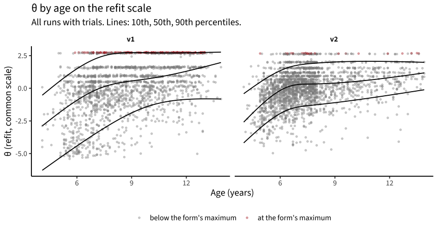
refit <- rf$scores |>filter(model =="g_estimated") |>left_join(runs |>select(run_id, dataset, age, time_started, layout), by ="run_id")refit |>filter(!is.na(age), age >=4, age <14) |>group_by(form) |>mutate(at_max = theta >=max(theta) -0.05) |>ungroup() |>ggplot(aes(age, theta)) +geom_point(aes(colour = at_max), alpha =0.35, size =0.9) +geom_quantile(quantiles =c(.1, .5, .9), formula = y ~ splines::ns(x, 3),colour ="black") +facet_wrap(~form) +scale_colour_manual(values =c(`FALSE`="grey55", `TRUE`="firebrick"),labels =c("below the form's maximum", "at the form's maximum"),name =NULL) +labs(x ="Age (years)", y ="θ (refit, common scale)",title ="θ by age on the refit scale",subtitle ="All runs with trials. Lines: 10th, 50th, 90th percentiles.") +theme(legend.position ="bottom")
Code
refit |>filter(!is.na(age)) |>group_by(form, age =age_band5(age)) |>summarise(runs =n(), sd =sd(theta), q10 =quantile(theta, .1),median =median(theta), q90 =quantile(theta, .9), .groups ="drop") |> knitr::kable(digits =2, caption ="θ by age and form on the refit scale")
θ by age and form on the refit scale
form
age
runs
sd
q10
median
q90
v1
<6
175
2.15
-4.82
-2.03
0.88
v1
6-8
646
2.08
-3.88
-0.19
2.67
v1
8-10
502
1.70
-1.74
0.48
2.70
v1
10-12
408
1.53
-1.13
0.96
2.73
v1
12+
178
1.54
-0.72
1.56
2.73
v2
<6
479
1.56
-3.41
-0.98
0.66
v2
6-8
1294
1.27
-1.50
0.26
1.95
v2
8-10
331
1.30
-1.23
0.41
1.99
v2
10-12
167
1.10
-0.87
0.71
1.74
v2
12+
132
1.17
-0.36
0.92
2.04
Code
refit |>filter(grepl("complete \\(", layout), !is.na(age)) |>group_by(form) |>mutate(form_max =max(theta)) |>group_by(form, age =age_band5(age)) |>summarise(runs =n(), at_max =mean(theta >= form_max -0.05),within_half_logit =mean(theta >= form_max -0.5), .groups ="drop") |>pivot_wider(names_from = form, values_from =-c(form, age)) |> knitr::kable(digits =3, caption ="Share of complete runs at, or within half a logit of, their form's maximum score")
Share of complete runs at, or within half a logit of, their form’s maximum score
age
runs_v1
runs_v2
at_max_v1
at_max_v2
within_half_logit_v1
within_half_logit_v2
<6
146
189
0.007
0.005
0.027
0.026
6-8
623
1028
0.045
0.014
0.119
0.056
8-10
482
281
0.075
0.007
0.160
0.075
10-12
404
150
0.124
0.013
0.290
0.053
12+
170
126
0.165
0.032
0.353
0.095
Code
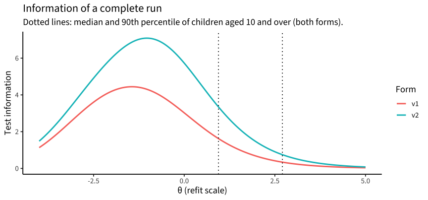
rf$info_curves |>filter(model =="g_estimated", theta >=-4, theta <=5) |>ggplot(aes(theta, info, colour = form)) +geom_line(linewidth =1) +geom_vline(xintercept =quantile(refit$theta[!is.na(refit$age) & refit$age >=10], c(.5, .9)),linetype ="dotted") +labs(x ="θ (refit scale)", y ="Test information",colour ="Form", title ="Information of a complete run",subtitle ="Dotted lines: median and 90th percentile of children aged 10 and over (both forms).")
Code
hf_test |>filter(form =="v1", !is.na(block), !is.na(age), age >=10) |>semi_join(complete_runs, by ="run_id") |>group_by(run_id) |>summarise(within_2s =all(correct %in%TRUE& rt_numeric >=200& rt_numeric <=2000),within_3s =all(correct %in%TRUE& rt_numeric >=200& rt_numeric <=3000),untimed =all(correct %in%TRUE& rt_numeric >=200), .groups ="drop") |>summarise(across(-run_id, mean)) |> knitr::kable(digits =2, caption ="v1 complete runs, ages 10+: share with every trial correct under three codings")
v1 complete runs, ages 10+: share with every trial correct under three codings
within_2s
within_3s
untimed
0.2
0.31
0.39
The ceiling falls. In v1, 12–17% of complete runs from children 10 and over sit at the form’s maximum, and 29–35% within half a logit of it. In v2 those shares are 1–3% and 5–10%. This comparison doesn’t depend on the anchors, since each form is compared with its own maximum. A complete v2 run also carries about twice the information of a v1 run at θ = 1–4 (part of that is the 16 extra mixed trials; per mixed trial the gain is about 1.4 times).
v1’s ceiling was also worse than the released scores show. Under the 2-s rule 20% of older v1 children make no errors; if every correct answer counts, 39% do. The released scoring hid half the ceiling by counting slow correct answers as errors.
But the range doesn’t widen. v2’s spread is narrower than v1’s at every age (SD 1.1–1.6 vs 1.5–2.2). At the bottom that is the feedback lifting the low end (§7). At the top, the v2 90th percentile sits below v1’s because v1’s top is a pile at the cap while v2’s is a spread of measured scores, but v2’s hardest items are still easier than most older children. The top is now resolved rather than stretched: older children are measured with more precision, within a narrower range.
Does the anchoring hold?
Using the pure blocks as anchors assumes they are equally difficult in both forms. Feedback could break that, since it changes how children recover from errors in exactly those blocks (§7). (The variance comparison above doesn’t depend on the anchors, because in a Rasch model each form’s variance is set by its own data. It does assume equal slopes across forms.) Three sites ran both forms in the same months, so their age-adjusted means should agree if the anchoring holds:
Code
concurrent <- refit |>filter(time_started >=as.POSIXct("2026-04-20", tz ="UTC"), !is.na(age)) |>group_by(dataset) |>filter(n_distinct(form) ==2, min(table(form)) >=10) |>ungroup()concurrent |>group_by(dataset) |>group_modify(\(x, ...) { m <-summary(lm(theta ~ form + age, data = x))$coefficientstibble(runs_v1 =sum(x$form =="v1"), runs_v2 =sum(x$form =="v2"),mean_age =mean(x$age),v2_minus_v1 = m["formv2", "Estimate"], se = m["formv2", "Std. Error"]) }) |>ungroup() |> knitr::kable(digits =2, caption ="Age-adjusted difference in refit θ (v2 − v1) at sites that ran both forms from April 2026")
Age-adjusted difference in refit θ (v2 − v1) at sites that ran both forms from April 2026
dataset
runs_v1
runs_v2
mean_age
v2_minus_v1
se
partner_mpib_de_main
78
16
6.98
0.40
0.44
pilot_western_ca_main
105
93
8.36
-0.02
0.25
rfp1_utdt_intl_ys
32
340
5.52
1.13
0.26
At Western (mean age 8.4) the two forms agree almost exactly. At UTDT’s young sample (mean age 5.5) v2 children score more than a logit higher. MPIB’s v2 sample is too small to say (16 runs; +0.40 ± 0.44). Either the anchors work differently for young children, which fits feedback helping them most in the pure blocks, or the two samples differ. So the common scale is reasonable from about age 7, and cross-form mean comparisons for younger children shouldn’t be trusted.
Verdict
Variants. The new form is taskVersion = 2, carried by every H&F variant created from 2026-04-23 (English (North America), es-AR, English (United Kingdom), German (Germany), Spanish (Colombia)); the 2025-07-21 variants are v1. Form follows the variant, not the code version, and several sites ran both concurrently.
The ding works as feedback (§7) but compresses the low end of the distribution. Keep it if the target construct is efficiency under conflict, not rule acquisition.
The floor nearly disappears and the ceiling falls, but the score range doesn’t widen (§4, §11). In a refit with the timed items calibrated separately, older children at their form’s maximum drop from 12–17% to 1–3%, and a complete v2 run gives about twice the information at high ability. But the hardest v2 item is still below the median 10-year-old, so the top is resolved rather than stretched, and v2’s spread is narrower than v1’s at every age. The faster segments act through timeouts, which also drive a large rise in early stops (~25% of v2 runs vs 5%) via the error-out rule.
No reliability gain: model-based reliability is about equal, split-half is lower, and cross-form retest at Leipzig is poor (.12, confounded with gap and age).
Shorter fixed windows won’t remove the ceiling on construct (§9). They do move items to the older children’s abilities (about 1.5 s for the median 10–12-year-old, about 1.25 s for the top decile), but the added difficulty is generic: the switch cost doesn’t grow, and in the counterfactual the score drifts from switching skill to plain speed. Measuring the top decile with this task means deciding that conflict resolution under time pressure is an acceptable construct for older children.
Neither scoring alternative helps (§10). A nominal model that separates timeouts from errors gives the same scores and the same reliability; imputing timeouts for stopped runs inflates internal consistency while slightly lowering external validity.
Recommendations for the DCC:
Score v1 and v2 as different forms. Same item uids are scored with one set of parameters, although v2 items differ in difficulty (deadlines, feedback). At minimum, add form-specific (or segment-specific) item uids and recalibrate; until then, don’t interpret θ change across the v1 → v2 boundary (e.g. Leipzig wave 3) as growth.
Align recode_hf() with the v2 windows. A 2000 ms cutoff inside a 3000 ms window scores coin-rewarded responses as errors. Either cut at the window or set the windows to 2 s.
Exempt timeouts from the error-out rule (or turn it off for H&F). That alone would have prevented 72% of v2’s early stops, mostly of young children. The rule’s comment and code also disagree (4 vs > 6 of 10).
Don’t use a 0.5 guessing floor for timed items. A missed window scores 0, not chance; calibrate each window separately with a lower or estimated floor, which also recovers information from trials already given.
Spend trials where the information is: shorten the pure blocks (they carry little information from about age 8 for hearts and 10 for flowers, but are useful as practice) and give the trials to mixed switch trials.
If the top decile must be measured, offer a ~1.25–1.5 s segment only to children who do well at 2 s, rather than to everyone; that adds information at the top without the young-child error-outs.
Keep scoring timeouts as errors in a dichotomous model, and don’t impute early stops: the score from the observed trials is already correct for a stopped run.
Plan a v2 → v2 retest before deciding on the redesign’s net value.