Memory (Corsi) — item difficulty structure & the ‘2×2 vs 3×3’ question
ImportantAI-generated — not for publication
The code and prose in this chapter were written by Claude Code (an AI coding agent) under human direction. They have not been line-by-line verified by a human and must not be published or cited as-is.
WarningPreliminary & unvetted analysis
These are exploratory analyses of preliminary, in-progress LEVANTE data. Results have not been reviewed or validated and require checking by the LEVANTE Data Coordinating Center before any use.
Question
The release notes flagged Memory scoring as not accounting for grid size (2×2 vs 3×3), and the task was marked DROP. But on corrected (v1.2) data the Colombia scores look fine, raising the hypothesis that the real culprit was the column-order scoring bug (now fixed) rather than the grid issue.
The Corsi span task has a clean design: sequences of squares light up and the child reproduces them. Each item is defined by three features encoded in item_uid (mg_{forward|backward}_{2grid|3grid}_len{N}):
direction — forward (same order) vs backward (reversed)
grid — 2×2 vs 3×3 (more locations ⇒ harder)
length — span length 2–7
We read the calibrated item difficulties as a function of these features — which reveals the actual difficulty structure of the task — and ask whether grid is properly separated and whether the structure replicates across sites.
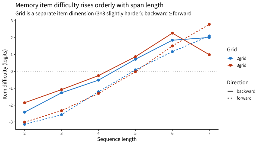
ip |>ggplot(aes(x = length, y = difficulty, color = grid, linetype = direction)) +geom_hline(yintercept =0, lty =3, color ="grey70") +geom_line(linewidth =0.9) +geom_point(size =2.5) +scale_color_manual(values =c(`2grid`="#268bd2", `3grid`="#cb4b16")) +scale_x_continuous(breaks =2:7) +labs(x ="Sequence length", y ="Item difficulty (logits)",title ="Memory item difficulty rises orderly with span length",subtitle ="Grid is a separate item dimension (3×3 slightly harder); backward ≥ forward",color ="Grid", linetype ="Direction")
Code
ip |>group_by(direction, grid) |>summarise(n_items =n(),cor_length_difficulty =cor(length, difficulty),logits_per_length =coef(lm(difficulty ~ length))[2],.groups ="drop") |> knitr::kable(digits =3,caption ="Difficulty is near-linear in length within each grid×direction")
Difficulty is near-linear in length within each grid×direction
direction
grid
n_items
cor_length_difficulty
logits_per_length
backward
2grid
6
0.988
0.936
backward
3grid
6
0.899
0.726
forward
2grid
6
0.996
1.106
forward
3grid
6
0.993
1.195
The span structure is exactly as a working memory task should behave: difficulty increases ~1 logit per added item, near-perfectly ordered (r ≈ 0.90–1.00). Backward spans are harder than forward at matched length.
2. Is grid size “accounted for”?
The release-notes concern was that scoring ignored 2×2 vs 3×3. But the items already separate by grid — each (direction, length) has distinct 2×2 and 3×3 items with their own calibrated difficulties.
Code
ip |>select(direction, length, grid, difficulty) |>pivot_wider(names_from = grid, values_from = difficulty) |>mutate(`3×3 − 2×2`=`3grid`-`2grid`) |>filter(!is.na(`3×3 − 2×2`)) |>arrange(direction, length) |> knitr::kable(digits =2, caption ="Grid effect at matched direction × length")
Grid effect at matched direction × length
direction
length
2grid
3grid
3×3 − 2×2
backward
2
-2.42
-1.86
0.56
backward
3
-1.27
-1.08
0.19
backward
4
-0.52
-0.25
0.27
backward
5
0.72
0.87
0.15
backward
6
1.85
2.27
0.42
backward
7
2.01
0.99
-1.02
forward
2
-3.14
-3.01
0.13
forward
3
-2.57
-2.33
0.24
forward
4
-1.21
-1.31
-0.10
forward
5
0.09
-0.02
-0.11
forward
6
1.17
1.51
0.34
forward
7
2.10
2.79
0.69
The 3×3 items are modestly harder than 2×2 at matched length (~+0.2–0.5 logits), as expected from the larger location set — and crucially this is captured in the item parameters, not lost. (The one large reversal is at length 7, where the 2×2 cell has very few responses.) So the “grid not accounted for” concern appears already handled by the item design; it is not what was breaking the scores.
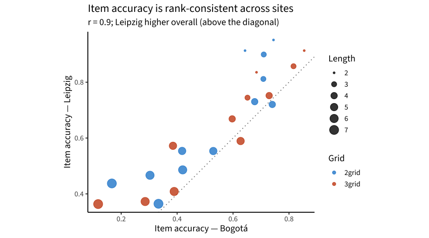
Item accuracies correlate r ≈ 0.90 across the two sites — the difficulty ordering is the same everywhere. Leipzig sits above the diagonal (higher accuracy), but that is a level difference (sample/age), not disorder or noise in the measure.
4. 2026-08 update: run-level comparability — sumscores vs IRT, and the grid question sharpened
Sections 1–3 established that grid is a calibrated item dimension. But the sharper comparability question is at the run level: in practice, runs are pure-grid — a child gets an all-2×2 or an all-3×3 administration (only 4 mixed runs among ~2,000), and grid assignment differs by site and wave (rural Colombia is ~99% 3×3; Leipzig and Bogotá are split). So no child ever links the two grids within a run, and cross-grid comparability rests entirely on the scoring model. Here we test it against model-free sumscores, exploiting the task’s staircase design: every run starts at length 2 and stops upward, so a span level the child never reached can be scored as failed — “imputing zeros for unreached steps” gives ladder scores that are well-defined across runs of different lengths.
Scored memory runs by grid × dataset — runs are pure-grid, and assignment is site- and wave-structured
dataset_label
runs_2grid
runs_3grid
mean_age_2grid
mean_age_3grid
Colombia — Bogotá
111
254
8.3
9.8
Colombia — Caquetá/Boyacá
6
419
4.8
10.1
Germany — Leipzig
258
286
9.1
9.0
Canada — Ontario
50
238
9.2
8.7
Germany — Berlin (MPIB)
3
147
7.8
7.2
US — LangCog (downext)
4
NA
4.1
NA
UK — Sheffield
1
17
9.7
7.6
Germany — MPIB (RfP1 YS)
9
69
4.8
5.9
US — Boston Children’s (downext)
7
3
4.6
5.3
4.1 Sumscores vs IRT θ
Code
cors <-function(d) tibble(n =nrow(d),total_correct =cor(d$score, d$ncorr),levels_passed =cor(d$score, d$levels_passed),max_span =cor(d$score, d$maxspan, use ="pair"))bind_rows(pooled =cors(mem), `2×2 runs`=cors(mem |>filter(grid =="2grid")),`3×3 runs`=cors(mem |>filter(grid =="3grid")), .id ="scope") |> knitr::kable(digits =3, caption ="Correlation of IRT θ with model-free sumscores")
Correlation of IRT θ with model-free sumscores
scope
n
total_correct
levels_passed
max_span
pooled
1882
0.880
0.889
0.898
2×2 runs
449
0.752
0.802
0.923
3×3 runs
1433
0.966
0.961
0.912
Within 3×3 runs, θ is nearly a rescaling of the sumscores (r ≈ 0.96); within 2×2 runs the correlation with total-correct is lower (r ≈ 0.75; max-span does better at 0.92), reflecting the 2×2 form’s compressed range and its concentration in the younger/earlier administrations. Ordering-wise, the model and the ladder agree.
4.2 The empirical grid test: Leipzig’s wave-1→2 grid switch
Leipzig switched most children from 2×2 (wave 1) to 3×3 (wave 2) at a ~5-month gap, while 42 children stayed 3×3→3×3 — a natural experiment for the model’s cross-grid linkage. If the linkage were wrong, the switchers would show a step in θ relative to the stayers.
Within-child change across Leipzig waves, by grid path
path
n
gap_yr
Δ θ
Δ levels
Δ max-span
2→3
168
0.42
0.15
2.20
-0.41
3→3
42
0.24
0.01
0.02
0.06
The sumscores expose their own non-comparability across the switch: max-span drops (−0.4) while levels-passed jumps (+2.2) for the same children — raw ladder scores mean different things on different boards. θ, by contrast, moves smoothly: switchers gain ≈ +0.15 over ~5 months while 3×3-stayers gain ≈ +0.01 over ~3 months — both consistent with modest within-year WM growth and with each other (≈ +0.3–0.4 θ/yr vs ≈ 0), with no step at the grid boundary. The model’s grid linkage passes the one empirical test the data afford.
One caveat stands: at matched levels-passed, pooled θ differs by grid by more than the ~0.3-logit item offsets alone would imply — but that comparison confounds grid with site and with the per-dataset EAP priors (2×2 runs live disproportionately in Leipzig/Bogotá wave 1). The switcher test above is the cleaner read, and it is reassuring.
Verdict (updated 2026-08)
Memory is well-behaved on corrected data. Difficulty is cleanly ordered by span length, backward > forward, and the structure replicates across sites (r ≈ 0.90).
The “2×2 vs 3×3” concern is handled at both levels. Grid is a separate calibrated item dimension (§2), and — the sharper run-level question — the model’s cross-grid linkage passes the Leipzig wave-1→2 switch test (§4.2): within-child θ is continuous across the grid change while raw sumscores visibly are not. Sumscores and θ agree on ordering (r ≈ 0.88–0.96).
Do not substitute raw sumscores across grids — max-span and ladder-total move in opposite directions across a grid switch; if a model-free score is ever needed, it must be within-grid only.
Recommendation: lift the DROP. Memory appears suitable for growth/SEM on the current (registry v2_3) scores. Residual caveats: the pooled grid-offset at matched sumscore partly reflects per-dataset EAP priors (not a pure item effect), and a few uncalibrated len8 trials should be excluded.