Hearts & Flowers — item structure (start/stay/switch) and 2PL vs Rasch

ImportantAI-generated — not for publication

The code and prose in this chapter were written by Claude Code (an AI coding agent) under human direction. They have not been line-by-line verified by a human and must not be published or cited as-is.

WarningPreliminary & unvetted analysis

These are exploratory analyses of preliminary, in-progress LEVANTE data. Results have not been reviewed or validated and require checking by the LEVANTE Data Coordinating Center before any use.

Question

Hearts & Flowers (inhibitory control / cognitive flexibility) has been through many scoring iterations. The most recent view: the nuanced item structure — distinguishing start / stay / switch trials within each block, and using a 2PL rather than a Rasch model — fits better. Here we check that on corrected (v1.2) data, and look at whether the structure replicates across sites (DE looked possibly noisier than CO).

Item structure (item_uid = {block}_{stim}_{type}):

  • block — hearts (congruent only), flowers (incongruent only), heartsflowers (mixed)
  • type — start (first trial of a block), stay (rule repeats), switch (rule changes; mixed block only)
Code
source(here::here("common.R"))
library(mirt)
ip <- load_item_parameters() |>
  filter(task_id == "hearts-and-flowers", subset == "all_items") |>
  mutate(block = str_extract(item_uid, "^(heartsflowers|hearts|flowers)"),
         type  = factor(str_extract(item_uid, "start|stay|switch"),
                        levels = c("start","stay","switch")),
         stim  = str_extract(item_uid, "heart|flower"))

1. Item difficulty and discrimination

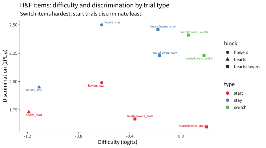
H&F is scored with a 2PL model, so each item has both a difficulty and a discrimination. The discrimination is where the action is.

Code
ip |> select(item_uid, block, type, difficulty, discrimination, n_responses) |>
  arrange(block, type) |>
  knitr::kable(digits = 2, caption = "H&F 2PL item parameters")
H&F 2PL item parameters
item_uid block type difficulty discrimination n_responses
flowers_flower_start flowers start -0.62 1.99 1571
flowers_flower_stay flowers stay -0.62 2.50 23382
hearts_heart_start hearts start -1.19 1.73 1572
hearts_heart_stay hearts stay -1.11 1.95 17153
heartsflowers_heart_start heartsflowers start 0.20 1.60 727
heartsflowers_flower_start heartsflowers start -0.36 1.67 830
heartsflowers_flower_stay heartsflowers stay -0.18 2.46 8768
heartsflowers_heart_stay heartsflowers stay -0.17 2.23 8808
heartsflowers_flower_switch heartsflowers switch 0.06 2.41 14911
heartsflowers_heart_switch heartsflowers switch 0.18 2.23 14999
Code
ip |>
  ggplot(aes(x = difficulty, y = discrimination, color = type, shape = block)) +
  geom_point(size = 3, alpha = 0.85) +
  ggrepel::geom_text_repel(aes(label = str_remove(item_uid, "_(heart|flower)")),
                           size = 2.6, show.legend = FALSE, max.overlaps = 20) +
  scale_color_brewer(palette = "Set1") +
  labs(x = "Difficulty (logits)", y = "Discrimination (2PL a)",
       title = "H&F items: difficulty and discrimination by trial type",
       subtitle = "Switch items hardest; start trials discriminate least")

Code
ip |> group_by(type) |>
  summarise(n = n(), mean_difficulty = mean(difficulty),
            mean_discrimination = mean(discrimination), .groups = "drop") |>
  knitr::kable(digits = 2, caption = "By trial type")
By trial type
type n mean_difficulty mean_discrimination
start 4 -0.49 1.75
stay 4 -0.52 2.29
switch 2 0.12 2.32

Two clear patterns:

  • Difficulty: pure blocks (hearts/flowers) are easy; the mixed block is harder, and switch trials are the hardest of all (the switch cost). This is the expected executive-function signature.
  • Discrimination: start trials discriminate least (a ≈ 1.75) vs. stay (≈ 2.28) and switch (≈ 2.32). Start trials are the first of a block — warm-up, noisier — so they carry less ability information. Forcing them to share a single discrimination (Rasch) misfits; giving them their own item label under a 2PL captures it.

2. 2PL vs Rasch

Code
tr <- load_levante_trials(task_ids = "hearts-and-flowers") |>
  filter(dataset %in% c("pilot_mpieva_de_main", "pilot_uniandes_co_bogota")) |>
  mutate(correct = as.numeric(correct))
wide <- tr |> distinct(run_id, item_uid, .keep_all = TRUE) |>
  select(run_id, item_uid, correct) |>
  pivot_wider(names_from = item_uid, values_from = correct) |>
  select(-run_id) |> as.matrix()
wide <- wide[, colMeans(!is.na(wide)) > 0.2]
wide <- wide[rowSums(!is.na(wide)) > 0, ]

m_rasch <- mirt(wide, 1, itemtype = "Rasch", verbose = FALSE)
m_2pl   <- mirt(wide, 1, itemtype = "2PL",   verbose = FALSE)
anova(m_rasch, m_2pl) |> as.data.frame() |>
  select(AIC, BIC, logLik, X2, df, p) |>
  knitr::kable(digits = 2, caption = "Rasch vs 2PL (pooled DE+CO)")
Rasch vs 2PL (pooled DE+CO)
AIC BIC logLik X2 df p
m_rasch 7810.49 7865.15 -3894.24 NA NA NA
m_2pl 7778.85 7878.23 -3869.42 49.64 9 0

The 2PL is preferred by the likelihood-ratio test (χ² ≈ 50, df = 9, p < .001) and AIC. (BIC is close, since the extra discrimination parameters are penalised heavily, but the LR test and the clear discrimination heterogeneity above favor 2PL.) This confirms the current scoring choice: start trials genuinely discriminate differently, and a 2PL is the right model.

3. Does the structure replicate across sites?

Code
acc <- tr |> group_by(dataset_label, item_uid) |>
  summarise(acc = mean(correct, na.rm = TRUE), .groups = "drop") |>
  left_join(ip |> select(item_uid, type, block), by = "item_uid") |>
  pivot_wider(names_from = dataset_label, values_from = acc)

acc |>
  ggplot(aes(x = `Colombia — Bogotá`, y = `Germany — Leipzig`, color = type)) +
  geom_abline(slope = 1, intercept = 0, lty = 3, color = "grey50") +
  geom_point(size = 3, alpha = 0.85) +
  scale_color_brewer(palette = "Set1") +
  coord_equal() +
  labs(x = "Item accuracy — Bogotá", y = "Item accuracy — Leipzig",
       title = "H&F item accuracy across sites",
       subtitle = glue::glue("r = {round(cor(acc$`Colombia — Bogotá`, acc$`Germany — Leipzig`, use='complete.obs'),2)}; consistent ordering, Bogotá slightly higher"))

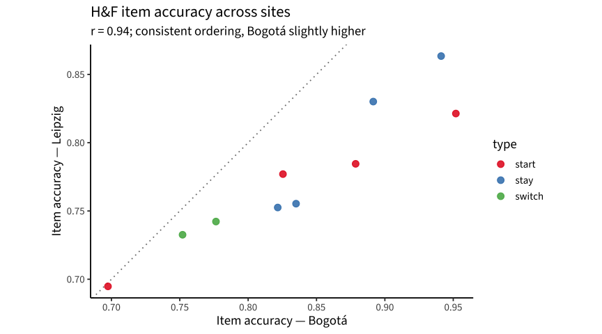
Item accuracies correlate r ≈ 0.94 across sites — the difficulty structure replicates. Here Bogotá is slightly higher-accuracy than Leipzig (the opposite direction from Memory, where Leipzig was higher), so there is no general “Leipzig is noisier” effect: each task’s site-level offset reflects sample/age, not measurement noise.

4. Ceiling effect

H&F scores pile up at a hard maximum. The question: is that just children who get literally nothing wrong?

Code
sc <- read_rds(here::here("data/scores_all_sites.rds"))
racc <- tr |> group_by(run_id) |>
  summarise(acc = mean(correct, na.rm = TRUE), n_items = n(), .groups = "drop")
hfc <- sc |> filter(task_id == "hearts-and-flowers", !is.na(score)) |>
  select(run_id, dataset_label, score) |> inner_join(racc, by = "run_id")
maxθ <- max(hfc$score, na.rm = TRUE)
hfc |> mutate(at_ceiling = score >= maxθ - 0.05) |>
  group_by(at_ceiling) |>
  summarise(n = n(), median_accuracy = round(median(acc), 3),
            min_accuracy = round(min(acc), 3),
            pct_perfect = round(mean(acc == 1) * 100, 1), .groups = "drop") |>
  knitr::kable(caption = glue::glue("Runs at the θ ceiling ({round(maxθ,2)}) all have perfect accuracy"))
Runs at the θ ceiling (1.68) all have perfect accuracy
at_ceiling n median_accuracy min_accuracy pct_perfect
FALSE 887 0.883 0 3.7
TRUE 56 1.000 1 100.0
Code
hfc |> group_by(dataset_label) |>
  summarise(n = n(),
            pct_perfect_accuracy = round(mean(acc == 1) * 100, 1),
            pct_at_theta_ceiling = round(mean(score >= maxθ - 0.05) * 100, 1),
            .groups = "drop") |>
  arrange(desc(pct_perfect_accuracy)) |>
  knitr::kable(caption = "Perfect-accuracy / ceiling rate by site")
Perfect-accuracy / ceiling rate by site
dataset_label n pct_perfect_accuracy pct_at_theta_ceiling
Germany — Leipzig 543 11.6 10.3
Colombia — Bogotá 400 6.5 0.0

Yes — the ceiling is exactly the children who make no errors. θ is capped at 1.68; every run there has 100% accuracy. About 10% of all runs are perfect-accuracy (they spread from θ ≈ 1 up to the cap depending on how many items they saw). The ceiling is worst in Canada (~16% perfect), then Germany (~12%), least in Colombia (~6%). The task simply lacks items hard enough to separate the strongest children — even the hardest switch trials sit at difficulty ≈ +0.1, well below where these kids are. A harder condition (tighter time limit or more demanding switch trials) would extend the ceiling.

Verdict

  • The start / stay / switch structure is psychometrically real: switch trials are hardest (switch cost), and start trials discriminate least (warm-up noise).
  • 2PL fits better than Rasch (LR + AIC), driven by that discrimination heterogeneity — the current scoring is right to model it.
  • Structure replicates across sites (r ≈ 0.94); site differences are level, not noise.
  • H&F looks usable on corrected data; the main subtlety to carry forward is that start trials are low-information (one could down-weight or drop them for a tighter ability estimate, but the 2PL already handles this).
Code
write_rds(ip, here::here("data", "hf_item_parameters.rds"))