08 — Accuracy variability: MSSD, the accuracy-level confound, and whether anything survives it
ImportantAI-generated — not for publication
The code and prose in this chapter were written by Claude Code (an AI coding agent) under human direction. They have not been line-by-line verified by a human and must not be published or cited as-is.
WarningPreliminary & unvetted analysis
These are exploratory analyses of preliminary, in-progress LEVANTE data. Results have not been reviewed or validated and require checking by the LEVANTE Data Coordinating Center before any use.
The question
07 showed RT intra-individual variability has a real (if narrow) signal once purified. This notebook is the accuracy companion. Accuracy is binary, so the RT tools (iSD, CV, ex-Gaussian) do not apply — the variability-indices tutorial (van Langen, Aristodemou & Kievit) flags MSSD (mean square of successive differences) as the index built for 0/1 data. For a binary sequence MSSD is just the trial-to-trial flip rate: how often the child switches right↔︎wrong on successive trials.
The central worry is a confound: for an independent Bernoulli sequence the flip rate is mechanically 2·p·(1−p), peaking at p = 0.5 and falling to 0 at floor/ceiling. So raw MSSD largely re-encodes accuracy level (≈ ability). We therefore compute three variants and — per the brief — carry the reliability and longitudinal-stability checks through to see which, if any, survives de-confounding:
raw MSSD — the flip rate (no correction)
detrended MSSD — flip-variability of residuals after removing the within-task trial-order trend (handles warm-up/fatigue, not accuracy level)
excess over independence — observed flip rate minus the child’s own independence expectation 2·p·(1−p) (handles accuracy level; equivalent to the scale-free lag-1 autocorrelation of the accuracy sequence)
Code
source(here::here("common.R"))library(splines)sc <-read_rds(here("data/scores_all_sites.rds"))sites4 <-c("pilot_mpieva_de_main","pilot_uniandes_co_bogota","pilot_uniandes_co_rural","pilot_western_ca_main")long_sites <-c("pilot_mpieva_de_main","pilot_uniandes_co_bogota","pilot_uniandes_co_rural")acc_tasks <-tibble(task_id =c("egma-math","matrix-reasoning","mental-rotation","trog","vocab","same-different-selection","hearts-and-flowers","theory-of-mind","memory-game","swr","sre","pa"),short =c("math","matrix","mrot","trog","vocab","sds","hf","tom","mg","swr","sre","pa"))adap <-c("egma-math","matrix-reasoning","mental-rotation","same-different-selection","trog","vocab")scor <-function(x, y){ ok <-is.finite(x) &is.finite(y)if (sum(ok) <3||sd(x[ok]) ==0||sd(y[ok]) ==0) return(NA_real_); cor(x[ok], y[ok]) }# per-run accuracy-variability indices for a task, given a set of runs (+ optional grouping col)acc_index <-function(tid, runs_tbl, extra =character()){ tr <-load_levante_trials(task_ids = tid) |>filter(run_id %in% runs_tbl$run_id, !is.na(correct), !is.na(trial_number)) |>left_join(runs_tbl |>select(run_id, all_of(extra)), by ="run_id") |>arrange(run_id, trial_number)if (nrow(tr) <150||n_distinct(tr$correct) <2) return(NULL) ns_ <-n_distinct(tr$dataset) form <-if (ns_ >1) correct ~ns(trial_number, 3) + dataset else correct ~ns(trial_number, 3) tr$phat <-predict(suppressWarnings(glm(form, binomial, tr)), type ="response") tr |>group_by(run_id) |>mutate(lc =lag(correct), resid = correct - phat, lresid =lag(resid),flip =as.numeric(correct != lc), dresid = resid - lresid,half =if_else(trial_number <=median(trial_number), 1L, 2L)) |>ungroup()}agg_run <-function(d, by =c("run_id")){ d |>group_by(across(all_of(by))) |>summarise(acc =mean(correct), ntrial =n(),raw =mean(flip, na.rm =TRUE),detrended =mean(dresid^2, na.rm =TRUE),excess =mean(flip, na.rm =TRUE) -2*mean(correct)*(1-mean(correct)),.groups ="drop") |>mutate(short =unique(d$short))}
1. Computing the index and the accuracy-level confound
Cross-sectional sample: first observation per child per task, four data-rich sites, newest (adaptive) version where one exists — the same frame as 07.
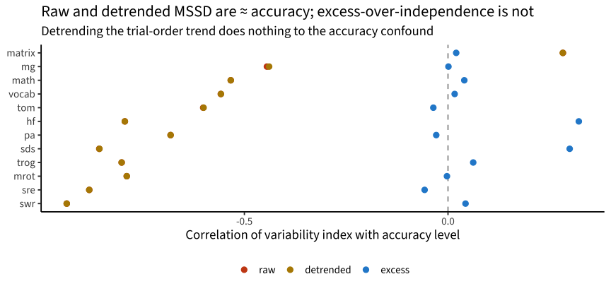
conf <- idx_xs |>group_by(short) |>summarise(raw =scor(raw, acc), detrended =scor(detrended, acc), excess =scor(excess, acc), .groups ="drop") |>pivot_longer(-short, names_to ="variant", values_to ="r")conf |>mutate(variant =factor(variant, c("raw","detrended","excess"))) |>ggplot(aes(r, reorder(short, r), color = variant)) +geom_vline(xintercept =0, linetype =2, color ="grey60") +geom_point(size =2.4) +scale_color_manual(values =c(raw ="#cb4b16", detrended ="#b58900", excess ="#268bd2"), name =NULL) +labs(x ="Correlation of variability index with accuracy level", y =NULL,title ="Raw and detrended MSSD are ≈ accuracy; excess-over-independence is not",subtitle ="Detrending the trial-order trend does nothing to the accuracy confound") +theme(legend.position ="bottom")
Raw MSSD correlates ≈ −0.7 with accuracy (more accurate children flip less), and detrending the trial-order trend changes this essentially nothing (raw ≈ detrended on every task) — the confound is the accuracy level, not a time trend. The excess-over-independence index removes it (confound ≈ 0): once we subtract each child’s own 2·p·(1−p) expectation, the flip rate is no longer a proxy for ability.
2. Does anything survive de-confounding? (reliability & stability)
The key test the brief asked for: do the de-confounded indices keep good internal reliability and longitudinal stability, or does removing the accuracy confound also remove the signal? Internal reliability uses a first-half/second-half split (MSSD is order-dependent, so odd/even would break the successive structure); stability is wave-1 vs wave-2 in the longitudinal samples (Leipzig + Bogotá).
Code
vars <-c("raw","detrended","excess")# internal reliability (first vs second half) on the cross-sectional samplerel_tab <-map_dfr(acc_tasks$short, function(s){ d <- trial_xs[[s]]; if (is.null(d)) return(NULL) hh <-agg_run(d, by =c("run_id","half")) |>filter(ntrial >=5)tibble(short = s, variant = vars, reliability =map_dbl(vars, function(v){ w <- hh |>select(run_id, half, val =all_of(v)) |>pivot_wider(names_from = half, values_from = val, names_prefix ="h") r <-scor(w$h1, w$h2); if (is.na(r)) NAelse2*r/(1+r) }))})# longitudinal test-retest (DE + Bogotá)wv <- sc |>filter(dataset %in% long_sites, task_id %in% acc_tasks$task_id, !is.na(score)) |>group_by(user_id, task_id) |>arrange(age) |>mutate(wave =row_number(), nwave =max(wave)) |>filter(nwave >=2, wave <=2) |>ungroup() |>select(run_id, user_id, task_id, short, wave) # sc already carries `short`ret_tab <-map_dfr(acc_tasks$task_id, function(tid){ s <- acc_tasks$short[acc_tasks$task_id == tid] d <-acc_index(tid, wv |>filter(task_id == tid), extra ="wave"); if (is.null(d)) return(NULL) pr <-agg_run(d, by =c("run_id","wave")) |>filter(ntrial >=10) |>left_join(wv |>select(run_id, user_id), by ="run_id")tibble(short = s, variant = vars, test_retest =map_dbl(vars, function(v){ w <- pr |>select(user_id, wave, val =all_of(v)) |>pivot_wider(names_from = wave, values_from = val, names_prefix ="w") |>filter(!is.na(w1), !is.na(w2)); scor(w$w1, w$w2) }))})perf <- rel_tab |>left_join(ret_tab, by =c("short","variant")) |>left_join(conf |>rename(acc_confound = r), by =c("short","variant"))
Across tasks: de-confounding (excess) trades away the reliable, stable signal
variant
mean |accuracy confound|
mean reliability
mean test–retest
raw
0.680
0.437
0.392
detrended
0.679
0.437
0.391
excess
0.077
0.035
0.063
Code
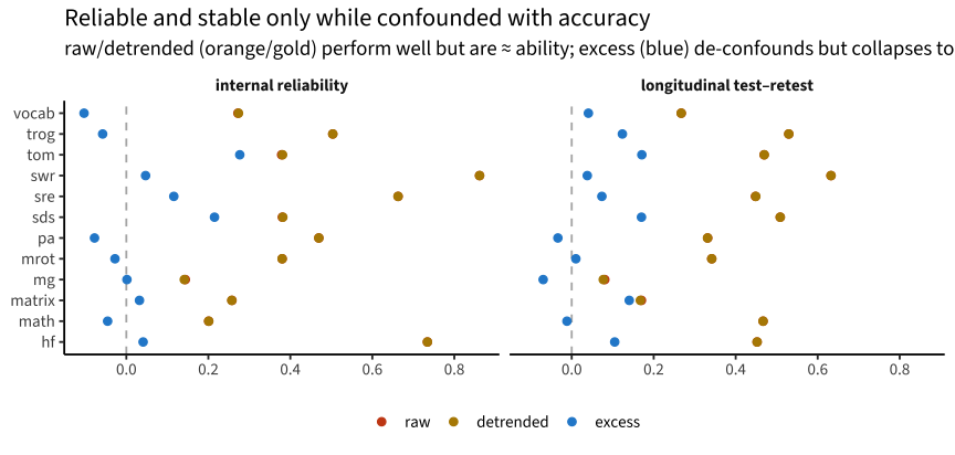
perf |>select(short, variant, reliability, test_retest) |>pivot_longer(c(reliability, test_retest), names_to ="metric", values_to ="value") |>mutate(variant =factor(variant, vars),metric =recode(metric, reliability ="internal reliability", test_retest ="longitudinal test–retest")) |>ggplot(aes(value, short, color = variant)) +geom_vline(xintercept =0, linetype =2, color ="grey70") +geom_point(size =2.2) +facet_wrap(~metric) +scale_color_manual(values =c(raw ="#cb4b16", detrended ="#b58900", excess ="#268bd2"), name =NULL) +labs(x =NULL, y =NULL, title ="Reliable and stable only while confounded with accuracy",subtitle ="raw/detrended (orange/gold) perform well but are ≈ ability; excess (blue) de-confounds but collapses to ~0") +theme(legend.position ="bottom")
This is the headline. Raw and detrended MSSD are reliably (≈ 0.44) and stably (test–retest ≈ 0.38) measured — on par with RT-IIV — but only because they re-encode accuracy (confound ≈ −0.7). The moment we remove the accuracy-level dependency, the excess index de-confounds (≈ 0) but its reliability falls to ≈ 0.03 and its stability to ≈ 0.02. There is essentially no stable, individual-differences signal in accuracy variability beyond accuracy level itself. (The scale-free lag-1 autocorrelation gives the same verdict.) This mirrors 06’s person-misfit result — once correctly de-confounded, “surprise”/instability in accuracy carries little reliable trait variance.
Does a better ability anchor (theta) rescue it?
The observed within-run proportion correct is a noisy ability anchor — and for adaptive tasks it is pinned near 0.5 regardless of ability. A principled alternative is to baseline against the IRT model’s predicted P per trial (from the child’s θ̂, item difficulty, and the fixed guessing asymptote the scoring uses), so the independence expectation reflects the actual item-difficulty sequence. We compare this theta-based excess to the observed-p excess on the longitudinal sample.
De-confounding baseline: observed p vs theta-IRF — neither leaves reliable signal
baseline
mean |confound w/ θ|
mean reliability
mean test–retest
observed p
0.104
0.016
0.057
theta-IRF predicted P
0.218
-0.167
0.145
It does not rescue the index. The theta-IRF baseline is, if anything, more confounded (≈ −0.2 vs +0.1) and has negative internal reliability (noise), with only a marginal, untrustworthy uptick in test–retest on a near-zero-reliability base — most likely because IRF miscalibration on some tasks (e.g. Same-&-Different, ROAR-Word) leaks ability back into the residual. The conclusion is therefore robust to the de-confounding method: by either a person’s own accuracy or a model-based θ̂ anchor, there is no stable accuracy-instability signal beyond ability.
3. Reliability vs trial count
Code
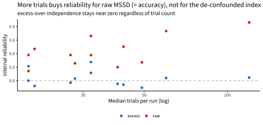
medn <- idx_xs |>group_by(short) |>summarise(median_trials =median(ntrial), .groups ="drop")rel_tab |>filter(variant %in%c("raw","excess")) |>left_join(medn, by ="short") |>ggplot(aes(median_trials, reliability, color = variant)) +geom_hline(yintercept =0, linetype =2, color ="grey70") +geom_point(size =2.3) +scale_x_continuous(trans ="log10") +scale_color_manual(values =c(raw ="#cb4b16", excess ="#268bd2"), name =NULL) +labs(x ="Median trials per run (log)", y ="internal reliability",title ="More trials buys reliability for raw MSSD (= accuracy), not for the de-confounded index",subtitle ="excess-over-independence stays near zero regardless of trial count") +theme(legend.position ="bottom")
For raw MSSD, reliability climbs with trial count (it inherits the reliability of the accuracy estimate). For the de-confounded excess index, more trials do not help — there is little true signal to estimate.
4. Cross-task structure
Code
mean_off <-function(cm) mean(cm[upper.tri(cm)], na.rm =TRUE)wide_v <-function(v) idx_xs |>select(user_id, short, val =all_of(v)) |>distinct(user_id, short, .keep_all =TRUE) |>pivot_wider(names_from = short, values_from = val)cmr <-cor(wide_v("raw") |>select(-user_id), use ="pairwise")cme <-cor(wide_v("excess") |>select(-user_id), use ="pairwise")tibble(structure =c("raw MSSD (≈ accuracy)","excess-over-independence"),`mean cross-task r`=round(c(mean_off(cmr), mean_off(cme)), 3)) |> knitr::kable(caption ="Raw MSSD coheres across tasks (it is ability/g); de-confounded does not")
Raw MSSD coheres across tasks (it is ability/g); de-confounded does not
structure
mean cross-task r
raw MSSD (≈ accuracy)
0.201
excess-over-independence
0.003
Raw accuracy-MSSD shows substantial cross-task coherence — but that is just the positive manifold of ability showing through (each task’s flip rate tracks its accuracy, and accuracies are intercorrelated). The de-confounded index shows near-zero cross-task structure, so there is no “accuracy-instability factor” analogous to the speeded RT-IIV factor.
5. Site and age
Code
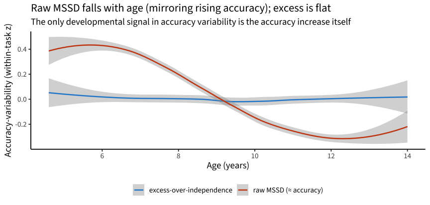
sa <- idx_xs |>left_join(sc |>distinct(run_id, dataset), by ="run_id") |>group_by(short) |>mutate(raw_z =as.numeric(scale(raw)), excess_z =as.numeric(scale(excess))) |>ungroup()bind_rows(sa |>transmute(age, value = raw_z, index ="raw MSSD (≈ accuracy)"), sa |>transmute(age, value = excess_z, index ="excess-over-independence")) |>ggplot(aes(age, value, color = index)) +geom_smooth(method ="loess", se =TRUE, linewidth =0.9) +scale_color_manual(values =c("raw MSSD (≈ accuracy)"="#cb4b16", "excess-over-independence"="#268bd2"), name =NULL) +labs(x ="Age (years)", y ="Accuracy-variability (within-task z)",title ="Raw MSSD falls with age (mirroring rising accuracy); excess is flat",subtitle ="The only developmental signal in accuracy variability is the accuracy increase itself") +theme(legend.position ="bottom")
Raw MSSD declines with age — but only because accuracy rises with age (so flips fall toward ceiling); the de-confounded index is flat. There is no developmental signal in accuracy instability once accuracy level is removed.
Synthesis
Accuracy variability is essentially ability in disguise. Raw and detrended MSSD are reliable, stable, age-graded, and cross-task coherent — but every one of those properties is inherited from accuracy level (confound ≈ −0.7; the flip rate is mechanically 2·p·(1−p)). Detrending the trial-order trend does not touch this.
Nothing reliable survives de-confounding. The excess-over-independence index (≡ lag-1 autocorrelation) cleanly removes the accuracy confound, but its reliability (≈ 0.03) and longitudinal stability (≈ 0.02) collapse to zero, and it shows no cross-task or age structure. There is no stable individual-difference trait of “accuracy instability beyond accuracy level” at these ages.
This parallels 06 and contrasts 07. It is the model-free confirmation of 06’s person-misfit result (de-confounded accuracy “surprise” ≈ 0 reliable signal). And it dissociates from RT: in 07, RT variability retained a real (if narrow, speeded-task) signal beyond mean RT, whereas accuracy variability retains nothing beyond accuracy level.
Practical recommendation. Do not treat accuracy MSSD as a variability measure — used raw it is an (inverse) ability score, and de-confounded it is noise. If within-child variability is the target, the leverage is in RT on speeded, high-trial tasks (07), not accuracy. (Faint exception: detrended accuracy autocorrelation on Hearts & Flowers shows a sliver of reliable, stable signal — consistent with H&F being the cleanest attentional-lapse task — but it is too weak to build on.)