Same & Different — scoring: IRTrees, chance floors, and a recommendation

ImportantAI-generated — not for publication

The code and prose in this chapter were written by Claude Code (an AI coding agent) under human direction. They have not been line-by-line verified by a human and must not be published or cited as-is.

WarningPreliminary & unvetted analysis

These are exploratory analyses of preliminary, in-progress LEVANTE data. Results have not been reviewed or validated and require checking by the LEVANTE Data Coordinating Center before any use.

NoteProvenance

Transferred from the SDS exploration in levante-pilots/03_explore_tasks/blockCAT/sds/ (data prep _recode_sds.R; modeling model_poly/, model_tree_lmer/, model_tree_mirt/), re-based here on the unified hackathon dataset. All artifacts are produced by tasks/_sds_scoring_fits.R and cached in data/sds_scoring/ — delete that directory to recompute (~35 min). Data: levante_data_pilots_hackathon:fpx0:v1_1 via the new levante package, cached by tasks/_pull_sds_hackathon.R.

source(here::here("common.R"))
suppressPackageStartupMessages({
  library(mirt); library(boot); library(knitr)
})
set.seed(42)

cache_dir <- here("data/sds_scoring")
if (!file.exists(file.path(cache_dir, "results.rds"))) {
  source(here("tasks/_sds_scoring_fits.R"))
}
coded <- read_rds(file.path(cache_dir, "coded.rds"))
tree <- read_rds(file.path(cache_dir, "tree.rds"))
audit <- read_rds(file.path(cache_dir, "audit.rds"))
mc <- read_rds(file.path(cache_dir, "mc.rds"))
bug <- read_rds(file.path(cache_dir, "bug.rds"))
res <- read_rds(file.path(cache_dir, "results.rds"))
factor_cors <- read_rds(file.path(cache_dir, "factor_cors.rds"))

raw <- read_rds(here("data/hackathon_v1_1_trials_sds.rds"))
runs_sds <- read_rds(here("data/hackathon_v1_1_scores.rds")) |>
  filter(task_code == "sds") |>
  select(run_id, user_id, dataset, age)
run_meta <- runs_sds |>
  left_join(raw |> group_by(run_id) |> summarise(t_start = min(timestamp)),
            by = "run_id")

The problem

SDS (“Same & Different Selection”) measures cognitive flexibility. In the match blocks (2match, 3match, 4match), a child sees k+1 cards containing exactly k matching pairs (each pair matching on a different dimension: size, color, shape, number, background). The child makes k successive pair selections: “find two that are the same” then, repeatedly, “find two that are the same in a different way.” A selection is credited correct if it is (a) a genuinely matching pair and (b) not a pair the child already chose in that trial.

This structure breaks the assumptions of our standard per-trial dichotomous IRT models in two ways:

1. Sequential dependence. What a child faces on selection 2 of a trial depends on what they did on selection 1. Both the chance level and the psychological demand (“shift to a new dimension”) are conditional on the response history.
2. Compound responses. “Correct” conflates two distinct behaviors: finding a match, and finding a new one (not perseverating on a previous choice).

Three approaches were explored in the original levante-pilots work:

• Polytomous (partial-credit) models over per-trial summed scores — rejected: collapsing the sequence into an ordinal count discards the conditional structure and produced disordered category thresholds.
• IRTree models via glmer (De Boeck & Partchev, 2012, JSS 48), decomposing each selection into sequential nodes — promising conceptually, but lmer random-effect scores don’t integrate with the mirt scoring pipeline.
• The same tree decomposition in mirt — evaluated here, against simpler item-structure alternatives.

The IRTree decomposition. Each selection is decomposed into up to two Bernoulli nodes:

• match: did the child select a matching pair (vs. non-matching)?
• new | match: given a match, was it a new pair (not previously selected)?
• new | non-match: given a non-match, was it at least a new error?

Because these nodes partition the outcome space, the likelihood factorizes cleanly and each node can be treated as a pseudo-item in an ordinary dichotomous IRT model — which is what makes this framework compatible with our mirt infrastructure. Nodes that are deterministic given the history (a “new” node when nothing has been selected yet, chance = 1; an “impossible new” node when all pairs of that type are exhausted, chance = 0) are dropped.

Data and recode

Match-block selections from all four pilot datasets, recoded from raw response/card-set strings by a direct port of the levante-pilots _recode_sds.R logic (trial boundaries reconstructed from choice1 markers, cross-validated against the “different” prompt text; trials dropped for empty/malformed responses, wrong selection counts, inconsistent card sets, or card sets that don’t afford exactly k matching pairs).

sel_n <- nrow(coded); run_n <- n_distinct(coded$run_id)
coded |>
  group_by(dataset) |>
  summarise(runs = n_distinct(run_id), selections = n(),
            `prop match` = mean(match), `prop correct` = mean(correct)) |>
  kable(digits = 2,
        caption = glue("{format(sel_n, big.mark = ',')} selections from {run_n} runs after recode"))

23,864 selections from 744 runs after recode

dataset	runs	selections	prop match	prop correct
pilot_mpieva_de_main	453	16834	0.95	0.80
pilot_uniandes_co_bogota	145	3186	0.91	0.64
pilot_uniandes_co_rural	19	669	0.78	0.51
pilot_western_ca_main	127	3175	0.91	0.73

Test–retest below uses the Leipzig (mpieva_de) children with two SDS administrations (~3- or ~7-month interval), scored per run from a single calibration.

The recode is verified correct

Because this recode is slated to be pushed upstream into levantemodels, it was audited with a fully independent reimplementation (regex token extraction instead of JSON parsing, direct attribute-table pair matching instead of the transpose/table helpers, independent trial sequencing and status counting; see the Recode B block of _sds_scoring_fits.R).

1. Stimulus grammar. All 142,921 stimulus tokens in every match-block response and card set parse as size-color-shape[-number][-texture] with the expected vocabularies (0 exceptions).

2. Cell-by-cell agreement between the two implementations:

audit$agreement |>
  select(`selections` = n, `match` = match_agree, `new` = new_agree,
         `correct` = correct_agree, `status (prev matches)` = status_m_agree,
         `status (prev non-matches)` = status_n_agree,
         `matching-pair count` = n_matches_agree) |>
  kable(digits = 4, caption = "Proportion agreement, independent reimplementation vs. pipeline recode")

Proportion agreement, independent reimplementation vs. pipeline recode

selections	match	new	correct	status (prev matches)	status (prev non-matches)	matching-pair count
23864	1	1	1	1	1	1

(A porting gotcha discovered during the original audit: trials must be indexed before dropping invalid responses — filtering rows first shifts trial indices whenever a dropped trial contains a choice1 row.)

3. Chance formulas. The conditional guessing formulas (\(P(\text{match}) = k/\binom{k+1}{2}\); \(P(\text{new} \mid \text{match}, m\text{ prior matches}) = 1 - m/k\); \(P(\text{new} \mid \text{non-match}, n\text{ prior non-matches}) = 1 - n/(\binom{k+1}{2} - k)\)) were verified by Monte Carlo simulation of the random-pair guessing process (30,000 simulated trials per block type; all simulated probabilities within simulation error of the formulas):

mc |>
  select(`k` = match_k, status, `P(match) MC` = p_match_mc,
         `P(match) formula` = p_match_formula,
         `P(new|M) MC` = p_newM_mc, `P(new|M) formula` = p_newM_formula,
         `P(new|N) MC` = p_newN_mc, `P(new|N) formula` = p_newN_formula) |>
  kable(digits = 3)

k	status	P(match) MC	P(match) formula	P(new|M) MC	P(new|M) formula	P(new|N) MC	P(new|N) formula
2	0m0n	0.664	0.667	1.000	1.000	1.000	1.000
2	0m1n	0.673	0.667	1.000	1.000	0.000	0.000
2	1m0n	0.663	0.667	0.495	0.500	1.000	1.000
3	0m0n	0.502	0.500	1.000	1.000	1.000	1.000
3	0m1n	0.496	0.500	1.000	1.000	0.664	0.667
3	0m2n	0.495	0.500	1.000	1.000	0.338	0.333
3	1m0n	0.505	0.500	0.662	0.667	1.000	1.000
3	1m1n	0.500	0.500	0.667	0.667	0.671	0.667
3	2m0n	0.486	0.500	0.342	0.333	1.000	1.000
4	0m0n	0.399	0.400	1.000	1.000	1.000	1.000
4	0m1n	0.402	0.400	1.000	1.000	0.837	0.833
4	0m2n	0.397	0.400	1.000	1.000	0.667	0.667
4	0m3n	0.402	0.400	1.000	1.000	0.492	0.500
4	1m0n	0.399	0.400	0.755	0.750	1.000	1.000
4	1m1n	0.390	0.400	0.754	0.750	0.828	0.833
4	1m2n	0.394	0.400	0.746	0.750	0.670	0.667
4	2m0n	0.406	0.400	0.487	0.500	1.000	1.000
4	2m1n	0.396	0.400	0.497	0.500	0.843	0.833
4	3m0n	0.409	0.400	0.264	0.250	1.000	1.000

Note these formulas are correct for the random-guessing model; whether that model is appropriate as an IRT floor is a separate question (Children are not random guessers, so theory-derived chance floors are misspecified — it is not).

A correctness bug in the production recode

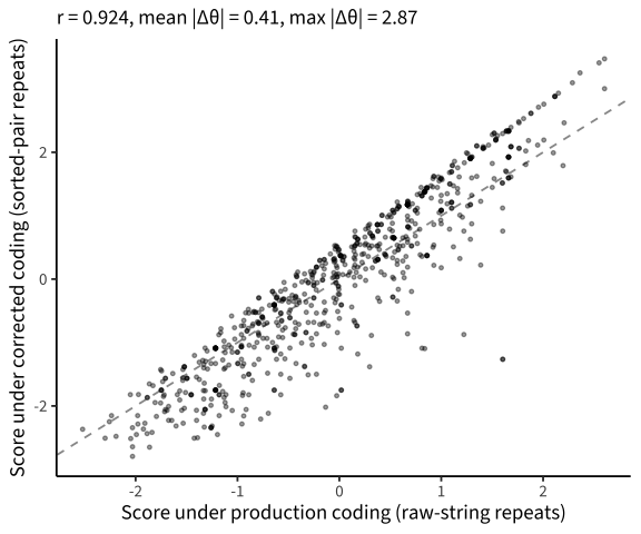
levantemodels::recode_sds() codes a selection as new iff its raw response string has not occurred earlier in the trial. But the response string records the two cards in selection order — so a child who re-selects the same pair in the opposite order produces a different string and is credited with a new (hence correct, if matching) response. The corrected recode sorts the parsed cards before comparison. This is not an edge case:

flipped <- bug$cmp |> filter(new_raw != new_sort)
tibble(
  `selections compared` = nrow(bug$cmp),
  `order-variant repeats (mis-credited as new)` = nrow(flipped),
  `% of selections` = round(100 * nrow(flipped) / nrow(bug$cmp), 1),
  `of which matching pairs (correct flips 1 to 0)` = sum(flipped$match),
  `runs affected` = n_distinct(flipped$run_id)
) |> kable()

selections compared	order-variant repeats (mis-credited as new)	% of selections	of which matching pairs (correct flips 1 to 0)	runs affected
23864	1536	6.4	1496	511

bs <- bug$bug_scores |> mutate(across(starts_with("theta"), as.numeric))
ggplot(bs, aes(x = theta_bug, y = theta_fix)) +
  geom_abline(linetype = "dashed", colour = "grey60") +
  geom_point(alpha = 0.4, size = 0.9) +
  labs(x = "Score under production coding (raw-string repeats)",
       y = "Score under corrected coding (sorted-pair repeats)",
       subtitle = glue("r = {round(cor(bs$theta_bug, bs$theta_fix), 3)}, ",
                       "mean |Δθ| = {round(mean(abs(bs$theta_bug - bs$theta_fix)), 2)}, ",
                       "max |Δθ| = {round(max(abs(bs$theta_bug - bs$theta_fix)), 2)}"))

EAP scores under the production (order-sensitive) vs. corrected repeat coding. Same model, same data, only the ‘new’ coding differs.

The fix (sorted-pair comparison) must land in levantemodels before any SDS model ships. Every analysis below uses the corrected coding.

Children are not random guessers, so theory-derived chance floors are misspecified

The LEVANTE convention is Rasch/2PL with a fixed guessing floor g = 1/#alts. The natural extension here sets each node’s floor from random pair-selection (the formulas above). But real children are not random: they perseverate, re-selecting previous pairs far more often than chance predicts. Several node-items sit below their theoretical floor, which a guessing-floor model cannot fit at all:

props <- tree |>
  summarise(prop = mean(value), n = n(), .by = c(node, item, chance)) |>
  mutate(below = prop < chance)
props |> filter(below) |> arrange(desc(n)) |>
  select(node, item, `chance floor` = chance, `observed prop` = prop, n) |>
  kable(digits = 2)

node	item	chance floor	observed prop	n
newM	3match_1m1n	0.67	0.64	147
newM	4match_1m1n	0.75	0.72	104
newN	4match_1m1n	0.83	0.61	54
newN	3match_0m1n	0.67	0.44	54
newM	4match_1m2n	0.75	0.60	20
newN	3match_0m2n	0.33	0.30	10
newN	4match_1m2n	0.67	0.60	10
newN	4match_0m1n	0.83	0.67	6
newN	4match_0m2n	0.67	0.00	2

share_below <- sum(props$n[props$below]) / sum(props$n)

1.1% of all node observations fall on below-floor items — concentrated in exactly the theoretically interesting “new” nodes. As shown below, the floors measurably reduce both internal and test–retest reliability, because they flatten the likelihood at the low end and discard stable individual variance in perseveration.

A framework for choosing the scoring model

The candidate space has four axes:

Axis	Options
Item structure	m0: block × choice (current production items, e.g. sds_2match_choice2) · m1: block × choice × response-history status (e.g. sds_2match_choice2_1m0n) · t: IRTree pseudo-items (match / new nodes × block × status)
Chance floors	theory-derived random-pair floors · none (g = 0)
Dimensionality	1 factor · 2–3 factors (match ability, “new”/shifting ability)
Item model	Rasch · 2PL

All models are fit in mirt on identical selections, with instance-constrained items (repeated encounters share parameters), N(0,3) difficulty priors, and N(1,0.3) slope priors for 2PL — matching the production pipeline’s conventions. The m0 variant labeled “corpus floors” uses the chance values currently in the corpus metadata (0.5 and 0.75 for 2match, 0 elsewhere), which match no principled guessing model.

Evaluation criteria, in the project’s priority order: (1) marginal/empirical reliability; (2) German test–retest r (bootstrap 95% CI); (3) age correlation as a validity proxy; (4) BIC, compared only among models of the same responses; (5) simplicity / pipeline fit.

Model comparison

scores_long <- res |>
  select(model, factor, scores) |>
  pmap(\(model, factor, scores) {
    scores |> select(run_id, value = all_of(factor)) |>
      # mirt >= 1.46 fscores columns can arrive as classed 1-col matrices
      mutate(value = as.numeric(value), model = model, factor = factor)
  }) |> list_rbind()
sum_scores <- coded |>
  group_by(run_id) |> summarise(value = mean(correct)) |>
  mutate(model = "sumscore", factor = "F1")
scores_long <- bind_rows(scores_long, sum_scores)
scored <- scores_long |> left_join(run_meta, by = "run_id")

age_cors <- scored |>
  summarise(r_age = cor(value, age, use = "complete.obs"), .by = c(model, factor))

retest_pairs <- scored |>
  filter(dataset == "pilot_mpieva_de_main") |>
  group_by(model, factor, user_id) |>
  filter(n() == 2) |>
  arrange(t_start, .by_group = TRUE) |>
  summarise(t1 = value[1], t2 = value[2], age1 = age[1], .groups = "drop")

boot_ci <- function(t1, t2, R = 2000) {
  b <- boot(tibble(t1, t2), \(d, i) cor(d$t1[i], d$t2[i], use = "complete.obs"), R = R)
  ci <- boot.ci(b, type = "perc")$percent[4:5]
  tibble(r_retest = b$t0, ci_lo = ci[1], ci_hi = ci[2])
}
retest_cors <- retest_pairs |>
  group_by(model, factor) |>
  summarise(boot_ci(t1, t2), n_retest = n(), .groups = "drop")

eval_table <- res |>
  select(model, factor, nfact, invariance, itemtype, converged,
         emp_rxx, marg_rxx, AIC, BIC, npar, logLik) |>
  bind_rows(tibble(model = "sumscore", factor = "F1")) |>
  left_join(age_cors, by = c("model", "factor")) |>
  left_join(retest_cors, by = c("model", "factor"))
n_retest <- retest_cors$n_retest[1]
fmt_retest <- \(r, lo, hi) glue("{sprintf('%.2f', r)} [{sprintf('%.2f', lo)}, {sprintf('%.2f', hi)}]")
gv <- function(m, col, f = "F1") eval_table[[col]][eval_table$model == m & eval_table$factor == f][1]

model_labels <- tribble(
  ~model, ~structure, ~floors, ~itemtype_l,
  "sumscore",  "proportion correct",      "—", "—",
  "m0_rasch",  "block × choice",          "corpus (production)", "Rasch",
  "m0_2pl",    "block × choice",          "corpus (production)", "2PL",
  "m0c_rasch", "block × choice",          "principled (mean)", "Rasch",
  "m0z_rasch", "block × choice",          "none", "Rasch",
  "m1_rasch",  "block × choice × status", "principled", "Rasch",
  "m1_2pl",    "block × choice × status", "principled", "2PL",
  "m1z_rasch", "block × choice × status", "none", "Rasch",
  "m1z_2pl",   "block × choice × status", "none", "2PL",
  "m1z_sig_rasch", "block × choice × status × features", "none", "Rasch",
  "t1_rasch",  "tree nodes, 1 factor",    "principled", "Rasch",
  "t1z_rasch", "tree nodes, 1 factor",    "none", "Rasch",
  "t1z_2pl",   "tree nodes, 1 factor",    "none", "2PL",
  "t2zc_rasch", "tree nodes, 2 corr. factors", "none", "Rasch",
  "t3z_rasch",  "tree nodes, 3 corr. factors", "none", "Rasch")

Pooled single-group models

All models converged. BIC is only comparable between models of the same responses: the selection universe (one Bernoulli response per selection: all m models) vs. the tree universe (each selection expanded into 1–2 node responses: all t models). The gate-augmented model (Adding feature-knowledge (“gate”) items helps) adds responses and is its own universe.

eval_table |>
  inner_join(model_labels, by = "model") |>
  mutate(universe = if_else(str_detect(model, "^t"), "tree", "selection"),
         retest = if_else(is.na(r_retest), NA,
                          fmt_retest(r_retest, ci_lo, ci_hi)),
         factor = if_else(factor == "F1", "", factor)) |>
  arrange(universe, BIC) |>
  select(universe, structure, floors, itemtype = itemtype_l, factor, BIC,
         `emp. rxx` = emp_rxx, `marg. rxx` = marg_rxx,
         `r (age)` = r_age, `retest r [95% CI]` = retest) |>
  kable(digits = 2)

universe	structure	floors	itemtype	factor	BIC	emp. rxx	marg. rxx	r (age)	retest r [95% CI]
selection	block × choice × status × features	none	Rasch		17400.43	0.85	0.90	0.31	0.52 [0.37, 0.64]
selection	block × choice × status	none	Rasch		17435.60	0.85	0.86	0.30	0.52 [0.38, 0.65]
selection	block × choice × status	none	2PL		17459.63	0.84	0.97	0.29	0.53 [0.40, 0.65]
selection	block × choice × status	principled	Rasch		17693.05	0.83	0.62	0.32	0.48 [0.32, 0.62]
selection	block × choice	none	Rasch		17736.64	0.82	0.82	0.29	0.51 [0.37, 0.64]
selection	block × choice × status	principled	2PL		17750.55	0.81	0.94	0.30	0.48 [0.34, 0.62]
selection	block × choice	principled (mean)	Rasch		17804.23	0.82	0.52	0.32	0.48 [0.33, 0.62]
selection	block × choice	corpus (production)	2PL		19170.31	0.72	0.93	0.32	0.58 [0.45, 0.68]
selection	block × choice	corpus (production)	Rasch		19288.29	0.72	0.78	0.32	0.59 [0.47, 0.70]
selection	proportion correct	—	—		NA	NA	NA	0.21	0.47 [0.30, 0.61]
tree	tree nodes, 2 corr. factors	none	Rasch	match	22051.64	0.62	NA	0.28	0.32 [0.12, 0.51]
tree	tree nodes, 2 corr. factors	none	Rasch	new	22051.64	0.84	NA	0.25	0.53 [0.39, 0.65]
tree	tree nodes, 3 corr. factors	none	Rasch	match	22052.32	0.62	NA	0.28	0.32 [0.13, 0.51]
tree	tree nodes, 3 corr. factors	none	Rasch	newM	22052.32	0.84	NA	0.25	0.54 [0.39, 0.66]
tree	tree nodes, 3 corr. factors	none	Rasch	newN	22052.32	0.30	NA	0.21	0.42 [0.26, 0.57]
tree	tree nodes, 1 factor	none	2PL		22897.58	0.84	0.97	0.27	0.52 [0.38, 0.64]
tree	tree nodes, 1 factor	none	Rasch		23358.54	0.85	0.90	0.30	0.51 [0.36, 0.64]
tree	tree nodes, 1 factor	principled	Rasch		24372.34	0.82	0.62	0.32	0.44 [0.27, 0.58]

Reading the table against the axes:

• Everything beats the sum score on validity (age r ≈ 0.3 for the IRT variants vs. 0.21 for proportion correct).
• Chance floors hurt. Within every item structure, removing the theory-derived floors raises test–retest reliability (status items: 0.48 with floors → 0.52 without; 1-factor tree: 0.44 → 0.51) and empirical reliability (0.83 → 0.85). This is the empirical footprint of Children are not random guessers, so theory-derived chance floors are misspecified. (The apparent retest advantage of the corpus-floors model, r = 0.59, is dissected in Why do the wrong production floors look good?.)
• Rasch wins BIC over 2PL and loses nothing (status items: 17,436 vs. 17,460), with equal-or-better empirical reliability and equivalent retest. The one criterion favoring 2PL — marginal reliability — is the least trustworthy: the 2PL’s model-implied information overstates its empirical reliability by 0.13, while the Rasch marginal and empirical values agree to 0.01. Simplicity says Rasch.
• Item structure matters less than expected for the score itself — with floors removed, all structures land at similar retest and age validity; status-aware structure buys a little empirical reliability, a clear BIC win over block × choice, and models the conditional difficulty honestly.
• Multi-factor trees split the construct, and only one factor holds up (What the tree decomposition teaches us): the match factor is unreliable and unstable, the newN factor is unmeasurable, and multidimensional multigroup models don’t fit the pipeline.

Why do the wrong production floors look good?

The strangest cell in the table: the model with the production corpus floors (g = .5 and .75 on the two 2match items, 0 elsewhere) — floors that match no guessing model — has the best nominal retest (0.59), beating both the correct guessing floors (0.48) and no floors (0.51). Three things are going on.

First, the statistics: the advantage is not established.

de_wide <- retest_pairs |>
  filter(model %in% c("m0_rasch", "m1z_rasch"), factor == "F1") |>
  select(model, user_id, t1, t2) |>
  pivot_wider(names_from = model, values_from = c(t1, t2)) |>
  drop_na()
b <- boot(de_wide, \(d, i) {
  d2 <- d[i, ]
  cor(d2$t1_m0_rasch, d2$t2_m0_rasch) - cor(d2$t1_m1z_rasch, d2$t2_m1z_rasch)
}, R = 4000)
ci <- boot.ci(b, type = "perc")$percent[4:5]

The bootstrap difference in retest r between the corpus-floors model and the recommended no-floor model is +0.07 [-0.00, +0.16] (n = 141 paired), and m0 is the maximum of 16 fitted models — winner’s curse can absorb much of the gap.

Second, the mechanism: a fixed guessing floor is not really a guessing parameter — it is an information reshaper. In a Rasch-with-guess model, \(P(\text{correct}) = g + (1-g)\,\sigma(\theta + d)\), two things happen as g rises: (i) the item’s information shrinks by roughly \((1-g)^2\), and (ii) the item becomes one-sided — a correct response is nearly uninformative, while an error remains strongly diagnostic of low ability. The corpus floors apply this surgery to exactly one block:

info_share <- function(mod_name) {
  mod <- read_rds(file.path(cache_dir, paste0("fit_", mod_name, ".rds")))
  th <- matrix(seq(-2, 2, length.out = 9))
  items <- extract.mirt(mod, "itemnames")
  ii <- map_dbl(items, \(it) mean(iteminfo(extract.item(mod, it), th)))
  tibble(item = items, info = ii, block = str_extract(items, "[0-9]match")) |>
    group_by(block) |> summarise(info = sum(info), .groups = "drop") |>
    mutate(share = info / sum(info), model = mod_name)
}
bind_rows(info_share("m0_rasch"), info_share("m0z_rasch")) |>
  mutate(model = fct_recode(model, "corpus floors (m0)" = "m0_rasch",
                            "no floors (m0z)" = "m0z_rasch")) |>
  select(model, block, share) |>
  pivot_wider(names_from = block, values_from = share) |>
  kable(digits = 3, caption = "Share of test information by block (θ ∈ [−2, 2])")

Share of test information by block (θ ∈ [−2, 2])

model	2match	3match	4match
corpus floors (m0)	0.032	0.450	0.519
no floors (m0z)	0.199	0.374	0.427

Third, 2match is exactly the block you’d want muted for this criterion. It is the near-ceiling warm-up block — and its choice2 item sits below its own .75 corpus floor, the same pathology as the tree nodes in Children are not random guessers, so theory-derived chance floors are misspecified — and its block-level sum score is the least stable of the three:

coded |>
  mutate(item_uid = glue("sds_{item_group}_{item_choice}")) |>
  filter(item_group == "2match") |>
  group_by(item_choice) |>
  summarise(`prop correct` = mean(correct), n = n(), .groups = "drop") |>
  mutate(`corpus floor` = c(0.5, 0.75)) |>
  kable(digits = 2, caption = "2match collapsed items vs. their corpus floors")

2match collapsed items vs. their corpus floors

item_choice	prop correct	n	corpus floor
choice1	0.97	5245	0.50
choice2	0.64	5245	0.75

block_props <- coded |>
  group_by(run_id, item_group) |>
  summarise(prop = mean(correct), .groups = "drop") |>
  left_join(run_meta, by = "run_id")
block_props |>
  group_by(item_group) |>
  summarise(`mean prop correct` = mean(prop),
            `r (age)` = cor(prop, age, use = "complete.obs"), .groups = "drop") |>
  left_join(
    block_props |> filter(dataset == "pilot_mpieva_de_main") |>
      group_by(item_group, user_id) |> filter(n() == 2) |>
      arrange(t_start, .by_group = TRUE) |>
      summarise(t1 = prop[1], t2 = prop[2], .groups = "drop") |>
      group_by(item_group) |>
      summarise(`retest r` = cor(t1, t2), `n retest` = n(), .groups = "drop"),
    by = "item_group") |>
  kable(digits = 2, caption = "Block-level sum-score properties")

Block-level sum-score properties

item_group	mean prop correct	r (age)	retest r	n retest
2match	0.79	0.25	0.41	141
3match	0.74	0.34	0.61	101
4match	0.65	0.23	0.18	14

2match content is also mostly match-node behavior — the unstable component from the tree analysis (What the tree decomposition teaches us) — because with only 3 cards the “new” demand is minimal.

So the wrong floors accidentally implement a defensible design decision — “treat the easy warm-up block as a low-end error detector and score the mid/high range from 3/4match” — through an indefensible mechanism. Like-for-like checks show no magic left once you see this: simply dropping 2match from the recommended model changes its retest by +0.020 on the common retest subsample, and the residual m0 edge is within the bootstrap noise above. The principled versions of the same move are already in the recommended model: the gate items supply calibrated low-end error detection with floors that are correct for genuine multiple-choice items (Adding feature-knowledge (“gate”) items helps), and 2PL — if we wanted it — learns a mild version of the block reweighting from data.

One genuine design implication for block-adaptive testing: for children in the retest age range, 2match contributes little stable signal, making it a natural candidate for age-gating or adaptive block skipping — while remaining essential floor coverage for younger/struggling children, which is precisely why it should stay in the calibrated item bank rather than be deleted.

What the tree decomposition teaches us

Even though the tree doesn’t win as a scoring model, it is diagnostic gold: it shows where the reliable signal in SDS lives. The table pools the 2-factor model (match, new) with correlated factors and the full 3-factor model that additionally splits new-given-match (newM) from new-given-non-match (newN).

eval_table |>
  filter(model %in% c("t2zc_rasch", "t3z_rasch")) |>
  mutate(model = fct_recode(model, "2-factor (match, new)" = "t2zc_rasch",
                            "3-factor (match, newM, newN)" = "t3z_rasch")) |>
  select(model, factor, `emp. rxx` = emp_rxx, `r (age)` = r_age,
         `retest r` = r_retest) |>
  kable(digits = 2)

model	factor	emp. rxx	r (age)	retest r
2-factor (match, new)	match	0.62	0.28	0.32
2-factor (match, new)	new	0.84	0.25	0.53
3-factor (match, newM, newN)	match	0.62	0.28	0.32
3-factor (match, newM, newN)	newM	0.84	0.25	0.54
3-factor (match, newM, newN)	newN	0.30	0.21	0.42

Three lessons:

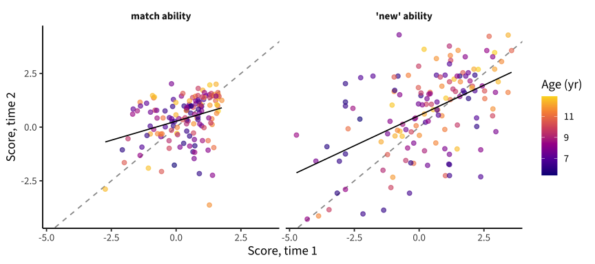
The “new” component carries the stable signal. Resisting perseveration and shifting to an unused pair has retest r ≈ 0.53 — on par with the best unidimensional models — while the match component is much noisier (rxx = 0.62, retest = 0.32). This makes psychological sense: with k matching pairs among k+1 cards, finding some match is easy and near ceiling for most children; the executive demand is in tracking what you already used and shifting dimensions. It also explains why item structure barely moves the overall score: however you slice the items, the stable variance comes from the same “new” behavior.

Match and “new” are close to distinct abilities. With the factor covariance freed, they correlate only r = 0.26. A single SDS θ is therefore a blend of two nearly orthogonal skills, weighted by item information — worth remembering when interpreting the score as “cognitive flexibility.”

The 3-node split adds nothing measurable. The 3-factor model converges and its BIC essentially ties the 2-factor model (22,052 vs. 22,052), but the newN factor rests on only 235 responses in the whole dataset (non-matches are rare outside 2match, where the newN node is deterministic and dropped) — so it is unmeasurable as an individual difference (rxx = 0.3). Its factor correlations are still informative: newN correlates with newM at r = 0.56 and with match at r = 0.03 — not repeating errors and not repeating successes share a common perseveration-resistance core that is unrelated to match-finding. Verdict: use the 2-factor tree for diagnostics; the 3-node split is theoretically tidy but empirically empty at these sample sizes.

A practical corollary: don’t discard newN nodes from the score. Under the floor model they look “below chance” and useless; without floors they contribute genuine signal about perseveration.

retest_pairs |>
  filter(model == "t2zc_rasch") |>
  mutate(factor = fct_recode(factor, "match ability" = "match",
                             "'new' ability" = "new")) |>
  ggplot(aes(x = t1, y = t2)) +
  facet_wrap(vars(factor)) +
  geom_abline(linetype = "dashed", colour = "grey60") +
  geom_point(aes(colour = age1), alpha = 0.6) +
  geom_smooth(method = "lm", se = FALSE, colour = "black", linewidth = 0.6) +
  scale_colour_viridis_c(option = "plasma", end = 0.92) +
  labs(x = "Score, time 1", y = "Score, time 2", colour = "Age (yr)")

German test–retest scores for the two tree factors (correlated 2-factor tree, no floors). The ‘new’ factor is substantially more stable.

Multigroup models: invariance ladder and sensitivity

The production pipeline fits multigroup models by site. Two questions: (a) which invariance level do the data support, and (b) does the multigroup setting change any pooled conclusion? (Multigroup filtering drops items not shared by all sites, so these BICs are not comparable with the pooled table.)

eval_table |>
  filter(str_detect(model, "^mg_m1z_(rasch|2pl)")) |>
  arrange(itemtype, desc(invariance)) |>
  select(itemtype, invariance, converged, npar, AIC, BIC,
         `emp. rxx` = emp_rxx, `r (age)` = r_age, `retest r` = r_retest) |>
  kable(digits = 2, caption = "Invariance ladder (status items, no floors, by site)")

Invariance ladder (status items, no floors, by site)

itemtype	invariance	converged	npar	AIC	BIC	emp. rxx	r (age)	retest r
2PL	scalar	TRUE	48	15717.87	15939.25	0.84	0.29	0.51
2PL	metric	TRUE	88	15665.10	16070.96	0.81	0.25	0.51
2PL	configural	TRUE	132	15736.64	16345.43	0.81	0.26	0.51
Rasch	scalar	TRUE	27	15764.90	15889.43	0.85	0.29	0.50
Rasch	configural	TRUE	69	15730.85	16049.08	0.82	0.26	0.50

Scalar invariance is the BIC-preferred level for both Rasch and 2PL, and Rasch-scalar beats 2PL-scalar overall. A likelihood-ratio test rejects exact scalar invariance against configural (as it essentially always does at these sample sizes), so there is some real cross-site DIF; but the parsimony judgment the pipeline applies elsewhere (BIC) lands on scalar, and scores are essentially insensitive to the level. Refitting the main structural contrast (m0z vs. m1z vs. t1z, Rasch, scalar-by-site) leaves every pooled conclusion intact:

eval_table |>
  filter(model %in% c("mg_m0z_rasch_scalar", "mg_m1z_rasch_scalar",
                      "mg_t1z_rasch_scalar")) |>
  mutate(structure = fct_recode(model,
    "block × choice (multigroup scalar)" = "mg_m0z_rasch_scalar",
    "block × choice × status (multigroup scalar)" = "mg_m1z_rasch_scalar",
    "tree nodes, 1 factor (multigroup scalar)" = "mg_t1z_rasch_scalar"),
    retest = fmt_retest(r_retest, ci_lo, ci_hi)) |>
  select(structure, `emp. rxx` = emp_rxx, `r (age)` = r_age,
         `retest r [95% CI]` = retest) |>
  kable(digits = 2)

structure	emp. rxx	r (age)	retest r [95% CI]
block × choice (multigroup scalar)	0.83	0.27	0.50 [0.35, 0.63]
block × choice × status (multigroup scalar)	0.85	0.29	0.50 [0.36, 0.63]
tree nodes, 1 factor (multigroup scalar)	0.84	0.28	0.49 [0.34, 0.62]

Binary experiments on the leading model

Adding feature-knowledge (“gate”) items helps

The SDS task opens with warm-up blocks excluded from all prior scoring: same (pick the card that is the same as a target; 2AFC) and dimensions (identify a card’s value on a named dimension; 3–4AFC). Conceptually these are a gate on the match blocks — a child who can’t identify the features can’t find feature matches — and they are near ceiling, so they carry information mainly about the low end of the scale. Every run in the match-block data also has gate trials, so adding them as ordinary dichotomous items costs nothing.

To be explicit about the guessing convention, since it differs by item type by design: gate items keep their standard multiple-choice floors (same g = .5; dimensions g = .25, or .33 for size), because they are genuine simultaneous forced choices where random selection is a coherent floor model and nothing pushes children below it (all gate items sit far above chance empirically). The match items get g = 0, because their “guessing” process is refuted by the data — children perseverate below the random-pair floor (Children are not random guessers, so theory-derived chance floors are misspecified). Mixed floors within one model are fully supported by the pipeline (chance is a per-item column).

eval_table |>
  filter(model %in% c("m1z_rasch", "m1z_gate_rasch",
                      "mg_m1z_gate_rasch_scalar")) |>
  mutate(model = fct_recode(model,
    "match blocks only (m1z, pooled)" = "m1z_rasch",
    "+ gate items (pooled)" = "m1z_gate_rasch",
    "+ gate items (multigroup scalar)" = "mg_m1z_gate_rasch_scalar"),
    retest = fmt_retest(r_retest, ci_lo, ci_hi)) |>
  select(model, `emp. rxx` = emp_rxx, `r (age)` = r_age,
         `retest r [95% CI]` = retest) |>
  kable(digits = 2)

model	emp. rxx	r (age)	retest r [95% CI]
match blocks only (m1z, pooled)	0.85	0.30	0.52 [0.38, 0.65]
+ gate items (pooled)	0.87	0.35	0.54 [0.40, 0.67]
+ gate items (multigroup scalar)	0.87	0.34	0.53 [0.37, 0.66]

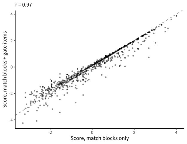
Adding gate items improves every criterion — empirical reliability, retest, and (largest of any manipulation tested) the age correlation, from 0.3 to 0.35. (BIC is not comparable — the model scores additional responses.) The gate-augmented model also converges as a multigroup scalar model, with scalar again BIC-preferred over configural (20,900 vs. 21,111).

gate_cmp <- scores_long |>
  filter(model %in% c("m1z_rasch", "m1z_gate_rasch"), factor == "F1") |>
  select(run_id, model, value) |>
  pivot_wider(names_from = model, values_from = value)
ggplot(gate_cmp, aes(x = m1z_rasch, y = m1z_gate_rasch)) +
  geom_abline(linetype = "dashed", colour = "grey60") +
  geom_point(alpha = 0.4, size = 0.9) +
  labs(x = "Score, match blocks only", y = "Score, match blocks + gate items",
       subtitle = glue("r = {round(cor(gate_cmp$m1z_rasch, gate_cmp$m1z_gate_rasch, use = 'complete.obs'), 3)}"))

Scores with vs. without gate items (pooled Rasch). Gate items mostly re-order the bottom of the scale, where ‘did this child know the features at all?’ is informative.

One caveat: gate items are near ceiling, so their discrimination is concentrated where few children are — the gains are real but the items mostly sharpen the floor of the scale (which is exactly what a gate should do). If the task is revised, a couple of harder feature-identification items would strengthen this further.

scored |>
  filter(model == "mg_m1z_gate_rasch_scalar") |>
  ggplot(aes(x = age, y = value)) +
  geom_point(aes(colour = dataset), size = 0.8, alpha = 0.6) +
  geom_smooth(method = "lm", colour = "black", linewidth = 0.7) +
  scale_colour_ptol() +
  labs(x = "Age (years)", y = "SDS score (θ)", colour = "Dataset")

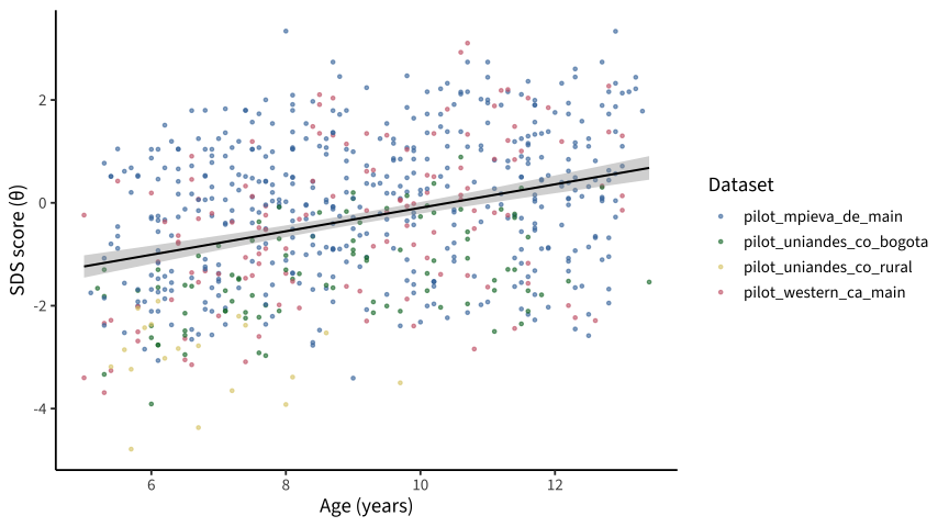
Recommended model (status-aware match items + gate items, no floors on match items, multigroup scalar Rasch): scores by age and dataset.

Disaggregating items by matched features does not help

The last level of item granularity: the specific dimensions in which a card set contains its matching pairs (e.g., a 2match set whose pairs match on color and size vs. one whose pairs match on shape and size). The deployed card sets realize only a few feature signatures per block, so items become block × choice × status × signature:

eval_table |>
  filter(model %in% c("m1z_rasch", "m1z_sig_rasch")) |>
  mutate(model = fct_recode(model, "status items (m1z)" = "m1z_rasch",
                            "status × feature-signature items" = "m1z_sig_rasch"),
         retest = fmt_retest(r_retest, ci_lo, ci_hi)) |>
  select(model, BIC, `emp. rxx` = emp_rxx, `r (age)` = r_age,
         `retest r [95% CI]` = retest) |>
  kable(digits = 2)

model	BIC	emp. rxx	r (age)	retest r [95% CI]
status items (m1z)	17435.60	0.85	0.30	0.52 [0.38, 0.65]
status × feature-signature items	17400.43	0.85	0.31	0.52 [0.37, 0.64]

There is systematic signature-level difficulty variation (same-universe BICs are comparable here), but reliability, retest, and age validity are unchanged — at the price of ~2.6× as many item parameters in the registry and items that depend on deployment-specific card sets. Not worth it for scoring; worth remembering if specific card sets ever need DIF screening.

Cross-stack check

This chapter re-derives, on the unified hackathon dataset, the analysis originally developed in levante-pilots on the four per-site processed datasets (24,799 selections / 811 runs / 168 retest pairs there). Headline numbers from that stack, for comparison with the tables above: status items no floors — rxx .845, age r .30, retest .50; with principled floors — retest .46; corpus-floors m0 — retest .56; + gate items — rxx .863, age r .35, retest .53; tree factors — match retest .36, new retest .51, factor r .24. Every qualitative conclusion — floors hurt, gate items help, Rasch ≥ 2PL, scalar invariance by BIC, “new” stable / match unstable, signatures useless — agrees across the two data stacks and the two recode implementations.

Recommendations

1. Port the (audited) corrected recode upstream into levantemodels::recode_sds() (The recode is verified correct, A correctness bug in the production recode). The repeat-detection fix (sorted-pair comparison) matters more than every modeling decision below. When porting, keep the trial-indexing order (index trials before dropping invalid responses).

2. Score SDS with status-aware dichotomous match items plus the same/dimensions gate items, no floors on the match items, Rasch, multigroup scalar. Concretely: item_uid = sds_{block}_{choice}_{status} (status = counts of previously used matching/non-matching pairs, e.g. 1m0n), correct = match & new, chance = 0 for match items; same and dimensions items enter as ordinary dichotomous items with their multiple-choice floors. This is the mg_m1z_gate row above — the best model on every criterion, converging cleanly in the production multigroup-scalar configuration.

3. Invariance: scalar, by the pipeline’s own standard — BIC-preferred at every rung tested, with scores insensitive to the level; DIF screening of the status items across sites remains good hygiene once the recode fix lands.

4. Correct the corpus chance metadata for SDS match items (currently 0.5/0.75/0 patterns that match no guessing model) — or make the no-floor choice explicit in the scoring spec so the metadata is ignored.

5. Keep the tree decomposition as a research/diagnostic tool. The correlated 2-factor tree shows SDS’s stable signal is perseveration-resistance (“new”), not match-finding, and that the two are nearly orthogonal. Worth (a) reporting as construct evidence, and (b) acting on if SDS is redesigned — more selections per trial, harder match discriminations, and a few harder feature-gate items would strengthen the weak components.

Limitations and open questions

• Test–retest is one site, two intervals (Leipzig, _3/7 months); scores come from a single calibration including both waves (standard for our pipeline, slightly optimistic vs. fixed-parameter scoring of wave 2).
• Gate items are scored with their released correctness — they don’t pass through the match-block recode; their answer keys deserve the same below-chance screening as other tasks before the combined model ships (nothing looked anomalous here).
• The tiny 3unique block (Bogotá only) remains excluded.
• Status-aware items condition on the child’s own response history, so item exposure is endogenous; the tree literature treats this as unproblematic for node-level measurement, but item parameters shouldn’t be interpreted as if statuses were randomly assigned.
• Guessing floors could in principle be estimated (3PL) rather than fixed or zeroed; with these sample sizes and the perseveration asymmetry, not worth the instability risk.