Stories (Theory of Mind) — consolidated analysis on the corrected 2026-09 data

ImportantAI-generated — not for publication

The code and prose in this chapter were written by Claude Code (an AI coding agent) under human direction. They have not been line-by-line verified by a human and must not be published or cited as-is.

WarningPreliminary & unvetted analysis

These are exploratory analyses of preliminary, in-progress LEVANTE data. Results have not been reviewed or validated and require checking by the LEVANTE Data Coordinating Center before any use.

Code
source(here::here("common.R"))

dir26 <- here("data/stories_2026-09")
res_items <- read_rds(file.path(dir26, "results_items.rds"))
res_mono  <- read_rds(file.path(dir26, "results_monotonicity.rds"))
res_dim   <- read_rds(file.path(dir26, "results_dimensionality.rds"))
res_inv   <- read_rds(file.path(dir26, "results_invariance.rds"))
res_rel   <- read_rds(file.path(dir26, "results_reliability.rds"))
trials    <- read_rds(file.path(dir26, "stories_trials.rds"))
runs      <- read_rds(file.path(dir26, "stories_runs.rds"))
recon     <- read_rds(file.path(dir26, "reconciliation.rds"))
dir2610   <- here("data/stories_2026-10")
res_nest  <- read_rds(file.path(dir2610, "results_nested.rds"))
res_fu    <- read_rds(file.path(dir2610, "results_followups.rds"))
relabels  <- read_csv(here("tasks/stories_qtype_relabels.csv"), show_col_types = FALSE)

# block-CAT design simulation (tasks/_stories_cat_sim.R)
res_cat <- read_rds(file.path(dir26, "results_cat_sim.rds"))
rule_labels <- c(random = "random", maxinfo = "max information", infomin = "information per minute",
                 rq2 = "top-2 randomesque", disc_a2 = "highest summed discrimination",
                 disc_mean = "highest mean discrimination", oracle = "information at true θ",
                 fixed = "fixed form")
cat_designs <- res_cat$designs |> select(design, design_label = label, n_stories, steps)
# mean realized reliability over the 8 calibration groups; minutes = median over groups
cat_grid <- res_cat$q1 |>
  group_by(design, n_stories, rule) |>
  summarise(rel = mean(rel_realized), med_min = median(median_min), q90_min = median(q90_min),
            max_exp = mean(max_exposure), .groups = "drop")
cg <- function(d, r, col = "rel") {
  x <- cat_grid[[col]][cat_grid$design == d & cat_grid$rule == r]
  stopifnot(length(x) == 1); x
}

# number formatting: n2(0.456) = ".46", n2(1.234) = "1.23"
n2  <- function(x, d = 2) sub("^(-?)0\\.", "\\1.", formatC(x, format = "f", digits = d))
pct <- function(x, d = 0) paste0(formatC(100 * x, format = "f", digits = d), "%")
big <- function(x) format(x, big.mark = ",", trim = TRUE)
rng <- function(x, d = 2) {
  lo <- min(x, na.rm = TRUE); hi <- max(x, na.rm = TRUE)
  paste0(n2(lo, d), if (lo < 0) " to " else "–", n2(hi, d))
}
fp  <- function(p) format.pval(p, digits = 2, eps = 1e-4)          # tables
pe  <- function(p) if (p < 1e-4) "< .0001" else paste("=", n2(p, 3))  # prose: "p `r pe(x)`"
spct <- function(x, d = 0) paste0(if_else(x > 0, "+", ""), pct(x, d))
options(knitr.kable.NA = "")
# pull exactly one value out of a results table (fails loudly otherwise)
pick <- function(df, col, ...) {
  x <- dplyr::filter(df, ...) |> dplyr::pull({{ col }})
  if (length(x) != 1) stop("pick(): expected 1 row, got ", length(x))
  x
}

# item labels: "tom_story4_deception_reality_check_2" -> "S4 rc_2"
short_entry <- function(e) e |>
  str_replace("false_belief", "fb") |> str_replace("reality_check", "rc") |>
  str_replace("emotion_reasoning", "er") |> str_replace("^reference", "ref")
uid_label <- function(uid) {
  m <- str_match(uid, paste0("story(\\d+)_(?:reality_known|moral_reasoning|interpretation|",
                             "deception|reference|second_order)_(.+?)(?:-\\d+)?$"))
  paste0("S", m[, 2], " ", short_entry(m[, 3]))
}

# palettes: languages borrow the colour of their main site in common.R's site_pal
lang_levels <- c("de-DE", "en-US", "en-GB", "es-CO", "es-AR")
lang_pal <- c("de-DE" = site_pal[["pilot_mpieva_de"]],
              "en-US" = site_pal[["pilot_western_ca"]],
              "en-GB" = site_pal[["rfp1_sheffield_gb"]],
              "es-CO" = site_pal[["pilot_uniandes_co"]],
              "es-AR" = site_pal[["rfp1_utdt_ar"]])
qtype_levels <- c("false_belief", "emotion_reasoning", "reference", "reality_check")
qtype_pal <- set_names(ptol_pal()(4), qtype_levels)

# dimensionality samples
dim_labels <- c(de_ib = "Leipzig item bank (de-DE)", de_ib_v2 = "Leipzig, V2 content only",
                de_ib_junelike = "Leipzig, June-style rebuild",
                wca_ib = "Western item bank (en-US)", bog_ib = "Bogotá item bank (es-CO)",
                bog_ib_nofb = "Bogotá, without story-1 FB",
                ar_nhb = "UTDT no-HA retest-B (es-AR)", ar_nhb_nofb = "UTDT, without story-13 FB")
dim_primary <- c("de_ib", "wca_ib", "bog_ib", "ar_nhb")
dim_pal <- c(de_ib = site_pal[["pilot_mpieva_de"]], wca_ib = site_pal[["pilot_western_ca"]],
             bog_ib = site_pal[["pilot_uniandes_co"]], ar_nhb = site_pal[["rfp1_utdt_ar"]])

small_groups <- res_rel$meta$small_groups   # < 25 runs: scored under the DE prior

# what PR #27 adds against the releases: restored trials vs mapped trials in newly included runs
k_add <- list(restored = sum(recon$added_by_kind$n[str_starts(recon$added_by_kind$kind, "restored")]),
              mapped = sum(recon$added_by_kind$n[recon$added_by_kind$kind == "mapped before, run newly included"]),
              flip_runs = sum(recon$run_flips$n[recon$run_flips$before == "few_valid_trials" &
                                                 recon$run_flips$after == "included"]))
stopifnot(k_add$restored + k_add$mapped == sum(recon$per_dataset$added))

# story lists as runs of consecutive numbers: c(2, 7:12) -> "2, 7–12"
story_ranges <- function(s) {
  s <- sort(unique(s)); brk <- c(0, which(diff(s) != 1), length(s))
  paste(map_chr(seq_len(length(brk) - 1), \(i) {
    r <- s[(brk[i] + 1):brk[i + 1]]
    if (length(r) > 1) paste0(r[1], "–", r[length(r)]) else as.character(r)
  }), collapse = ", ")
}

# dataset labels (common.R has no label for rfp1_mpib_de_main)
ds_label <- function(d) coalesce(unname(dataset_labels_named[d]), d)

Purpose and what changed since June

NoteUpdate, 2026-10-17

Three sections were added after a review by Rebecca Saxe, on the same 2026-09 data: corrected question types (the corpus entry names file moral judgments and knowledge-access questions under false belief; a relabel table for the team, and a test of whether story type matters beyond question type), why development looks flat in Leipzig and Colombia, and Argentina vs Colombia. Earlier sections still use the corpus labels.

This chapter consolidates the Stories (Theory of Mind, ToM) analyses on the newest data, with item identities corrected. It supersedes three June chapters, now retired to old/ in the source repository: structure, rescoring and item analysis (old/stories_tom.qmd), dimensionality (old/tom_dimensionality.qmd) and multigroup DIF (old/tom_dif_multigroup.qmd). The June forensic reconstruction stays as the appendix on how the early deployment defects were found. The section on the exclusion list below revises its account of what went wrong with each item.

The June chapters were frozen on 2026-07-16. They used the June v1_2 release (pilot sites only) and the v1_14 per-language scoring models. Since then, five things have changed:

  1. Data. Every raw site dataset with ToM runs, pinned on 2026-09-24: 3,095 included runs from 2,724 children, 78,005 trials, 10 datasets and 5 languages. The largest new sample is UTDT Argentina (es-AR), which runs only stories 13–18.
  2. Item identity. levantemodels PR #27 (unmerged) fixes item identities in three deployment epochs and sets chance per story question. Against the latest releases (for Sheffield, its unreleased next draft of 2026-09-24, which matches the pinned raw data) it adds 1,382 trials: 1,366 restored by PR #27 and 16 in 2 Bogotá runs that the restores lift above the 10-trial minimum. It relabels 1,435 and changes correct for 0 trials.
  3. Item policy. Items are excluded by story-level flags defined in the data build (tasks/_build_stories_data.R), not by the generic Airtable list. The Spanish reality_known false-belief items are a sensitivity set, analysed with and without. The flags are listed below; they are analysis choices, and the recommendations say where they should live.
  4. Scoring. Each dataset with at least 25 runs gets its own group mean and variance, as proposed in levantemodels PR #26 (unmerged). Here the groups are estimated in one concurrent calibration, on a wider integration grid than production uses.
  5. Methods. The reliability and invariance models fix the guessing floor at chance (the LEVANTE convention). The dimensionality models set it to 0 for items answered at or below chance, and the other two analyses are rerun under that rule as a check. Correlations are computed within dataset × form rather than pooled over sites. Reliability is reported as empirical (EAP) reliability of what children actually answered. Dimensionality uses a resampled parallel analysis and bifactor models.

Four analysis scripts produced the results this chapter reads (see Reproducing). The chapter itself fits no models.

Code
k <- list()
fs <- res_items$flag_summary$by_language
k$cells_ok      <- sum(fs$ok)
k$cells_ceiling <- sum(fs$ceiling)
k$cells_weak    <- sum(fs$weak)
k$cells_poor    <- sum(fs$poor)
k$cells_bcd     <- sum(fs$`below chance, discriminating`)
k$cells_flag    <- k$cells_ok + k$cells_ceiling + k$cells_weak + k$cells_poor + k$cells_bcd
k$acc_13_ar <- pick(res_items$items_lang, accuracy,
                    story_uid == "tom_story13_reality_known_false_belief", language == "es-AR")

vc <- res_items$verdict_counts
vcn <- \(v) sum(vc$n[vc$verdict == v])
k$v_es_disc <- vcn("un-exclude (below chance in Spanish, but discriminates)")
k$v_un   <- vcn("un-exclude") + vcn("un-exclude (weak item)") + k$v_es_disc
k$v_weak <- vcn("un-exclude (weak item)")
k$v_es   <- vcn("un-exclude; flag es-* in analyses, no Airtable row until the translation check")
k$v_scop <- vcn("scoped exclusion")
k$v_keep <- vcn("keep excluded")
k$v_all  <- sum(vc$n)
stopifnot(k$v_un + k$v_es + k$v_scop + k$v_keep == k$v_all)

cr <- res_items$construct_r2
k$r2_qt  <- pick(cr, R2, outcome == "difficulty (IRT, z within language)",
                 unit == "item x language", scheme == "question_type (4)")
k$r2_og  <- pick(cr, R2, outcome == "difficulty (IRT, z within language)",
                 unit == "item x language", scheme == "old_group (6)")
k$r2_nc  <- pick(cr, R2, outcome == "difficulty (IRT, z within language)",
                 unit == "item x language", scheme == "new_construct (6)")
slope_unit <- "item x language (language FE; dR2 over it)"
k$dr2_nc <- pick(cr, dR2, outcome == "age slope (logit per year)", unit == slope_unit,
                 scheme == "new_construct (6)")
k$p_nc   <- pick(cr, p, outcome == "age slope (logit per year)", unit == slope_unit,
                 scheme == "new_construct (6)")

eg <- res_dim$eigen
k$ev_de <- pick(eg, ev1_ev2, sample == "de_ib")
k$ev_other <- eg$ev1_ev2[eg$sample %in% setdiff(dim_primary, "de_ib")]
ld <- res_dim$irt_ld |> filter(family == "guess", sample %in% dim_primary)
k$ecv <- rng(ld$ECV); k$omh <- rng(ld$omega_h); k$cor_uni_g <- rng(ld$cor_theta_uni_general, 3)
k$info_over <- paste0(pct(min(ld$info_overstatement)), "–", pct(max(ld$info_overstatement)))
spec_signs <- res_dim$irt_slopes |>
  filter(family == "guess", has_story_factor, sample %in% dim_primary) |>
  group_by(sample, story) |>
  summarise(mixed = any(lambda_specific < 0) & any(lambda_specific > 0),
            sum_abs = sum(abs(lambda_specific)), abs_sum = abs(sum(lambda_specific)), .groups = "drop")
k$mixed_stories <- sum(spec_signs$mixed); k$n_story_factors <- nrow(spec_signs)
k$de_s2_abs <- pick(spec_signs, sum_abs, sample == "de_ib", story == 2)
k$de_s2_sum <- pick(spec_signs, abs_sum, sample == "de_ib", story == 2)

cc <- res_items$controls_cor
k$r_ct_pooled <- pick(cc, r_control_target, method == "pooled over runs (June method)",
                      item_set == "policy items dropped")
k$r_ct_within <- pick(cc, r_control_target, method == "within dataset x form, Fisher-pooled",
                      item_set == "policy items dropped")

dbt <- res_inv$dif_by_type
k$A_ctrl_x2  <- pick(dbt, share_of_s1_X2, analysis == "A", kind == "control")
k$A_ctrl_it  <- pick(dbt, share_of_items, analysis == "A", kind == "control")
k$B_ctrl_x2  <- pick(dbt, share_of_s1_X2, analysis == "B", kind == "control")
tst <- res_inv$tests
k$A_scal_x2df <- pick(tst, X2_df, analysis == "A", comparison == "scalar vs configural", items == "all")
k$B_scal_x2df <- pick(tst, X2_df, analysis == "B", comparison == "scalar vs configural", items == "all")
k$A_part_p <- pick(tst, p, analysis == "A", comparison == "partial scalar vs configural", items == "all")
k$B_part_p <- pick(tst, p, analysis == "B", comparison == "partial scalar vs configural", items == "all")

# reliability headline: aggregate fixed-form and fCAT rows per dataset
agg_forms <- c("fCAT", "all fixed forms", "all forms")
form_types <- res_rel$rel_by_form |> filter(!form %in% agg_forms) |> distinct(dataset, form_type)
single_type <- form_types |> count(dataset) |> filter(n == 1) |> pull(dataset)
rel_head <- bind_rows(
  res_rel$rel_by_form |> filter(form %in% c("all fixed forms", "fCAT")),
  res_rel$rel_by_form |> filter(form == "all forms", dataset %in% single_type) |>
    select(-form_type) |> left_join(form_types, by = "dataset")
) |>
  filter(!dataset %in% small_groups) |>
  mutate(kind = if_else(str_starts(form_type, "fCAT"), "fCAT (3 random stories)", "fixed forms"))
k$rel_fixed <- rng(rel_head$rel_empirical[rel_head$kind == "fixed forms"])
k$rel_fcat  <- rng(rel_head$rel_empirical[rel_head$kind != "fixed forms"])
# single fixed forms (dataset x form, >= 25 runs)
rel_forms <- res_rel$rel_by_form |>
  filter(form_type == "fixed form", !form %in% agg_forms, n_runs >= 25, !dataset %in% small_groups) |>
  arrange(rel_empirical)
form_lab <- \(r) paste0(ds_label(r$dataset), " ", r$form, ", ", r$n_runs, " runs")
k$low_form  <- form_lab(slice_head(rel_forms, n = 1))
k$high_form <- form_lab(slice_tail(rel_forms, n = 1))
k$rel_forms <- rng(rel_forms$rel_empirical)
dc  <- \(d, col) pick(res_rel$density_check, {{ col }}, dataset == d)
g0s <- \(d, col) pick(res_rel$g0_sensitivity, {{ col }}, dataset == d)
blk <- \(b) res_rel$fcat_blocks$story[res_rel$fcat_blocks$block == b]
cs  <- res_rel$cat_sim_summary
csv <- \(d, col) pick(cs, {{ col }}, dataset == d)
je <- res_rel$june_equivalents
k$de_bank <- pick(je, value, str_starts(quantity, "DE full-bank marginal"))
sb <- res_rel$stability_bins
k$stab_60 <- pick(sb, r, dataset == "pilot_mpieva_de_main", gap_bin == "[60,180)", version == "analysis")
k$stab_60_lo <- pick(sb, r_lo, dataset == "pilot_mpieva_de_main", gap_bin == "[60,180)", version == "analysis")
k$stab_60_hi <- pick(sb, r_hi, dataset == "pilot_mpieva_de_main", gap_bin == "[60,180)", version == "analysis")
jp <- res_dim$june_pool_check
k$fixed_items <- rng(rel_head$median_items[rel_head$kind == "fixed forms"], 0)
k$fcat_min    <- rng(rel_head$median_minutes[rel_head$kind != "fixed forms"], 1)
rc  <- res_rel$released_comparison |> filter(!dataset %in% c(small_groups, "all (pooled)"))
own <- res_rel$released_models |> filter(own_group_in_v2_3) |> pull(dataset)
k$shift_total <- rng(-rc$shift_analysis_minus_released[!rc$dataset %in% own], 1)
k$shift_prior <- rng(-rc$shift_own_minus_ref_prior[!rc$dataset %in% own], 1)

Summary

Code
# numbers the summary needs from later sections (computed here, where the summary is)
sum_q3 <- res_dim$q3_grouping_contrast |> filter(sample %in% dim_primary, grouping == "question type")
sum_st <- res_items$slope_tests
sum_fl <- \(col) pick(sum_st, {{ col }}, outcome == "slope_floor", scheme == "question_type")
sum_2pl <- \(a, col) pick(res_inv$tests_2pl, {{ col }}, analysis == a, comparison == "scalar vs metric")
sum_rasch <- \(a, col) pick(res_inv$tests, {{ col }}, analysis == a, comparison == "scalar vs configural", items == "all")
  • Item quality. Of the 327 item × language cells with at least 30 responses, 215 are fine, 49 are at ceiling, 41 discriminate weakly, 20 are poor and 2 are below chance but still discriminate. The poor cells are the policy-flagged content plus Spanish reality_known false-belief items (story 13 in es-AR: .235 correct with two response options).
  • The exclusion list. The 12 generic Airtable entries cover 28 story-level items. 20 of them should be un-excluded (1 weak; 2 below chance in Spanish but still discriminating). 3 need exclusions scoped to one content version; for the two on image 4g, a key correction is the alternative, if the content team confirms it. 4 should stay excluded everywhere: reference_reference in stories 5, 11 and 17, and story 10’s deception false belief 1, which does not discriminate. Story 13’s reality_known false belief keeps an analysis flag in Spanish, and any Airtable row for it should wait for the translation check. The scoped rows cannot be written in today’s Airtable schema.
  • Do higher scorers do better? Checked directly (top against bottom third on the other items), 64 of 92 items pass, and the screen finds the policy-flagged items on its own. Outside the flags, two fail with enough data: story 17’s emotion question (“How does Mom feel about not finding the book?”), where higher-scoring German children answer surprised, and story 2’s reality check 2 on the V0 Bogotá scene. The three reference questions are reversed or flat: children answer with what the speaker meant, more so the higher they score, and none is worth keeping as written.
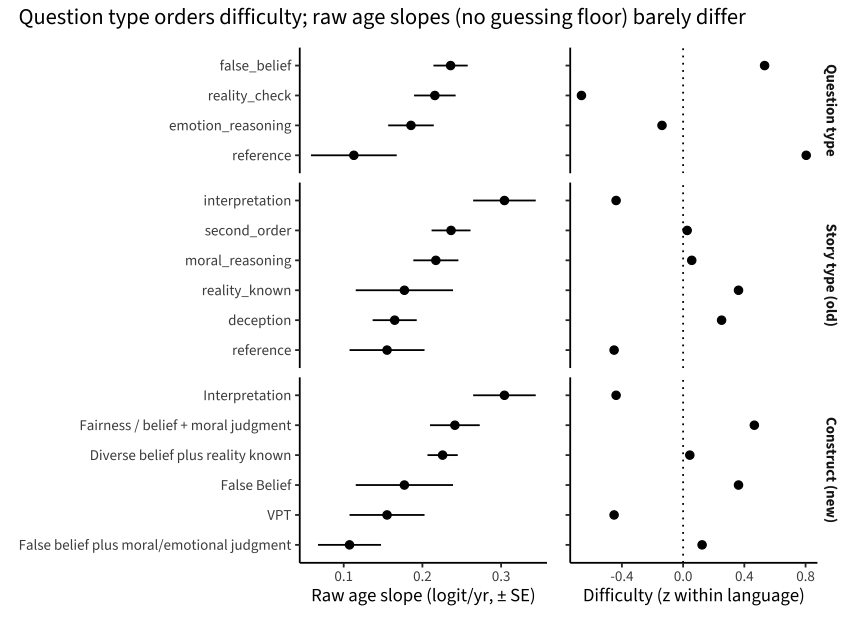
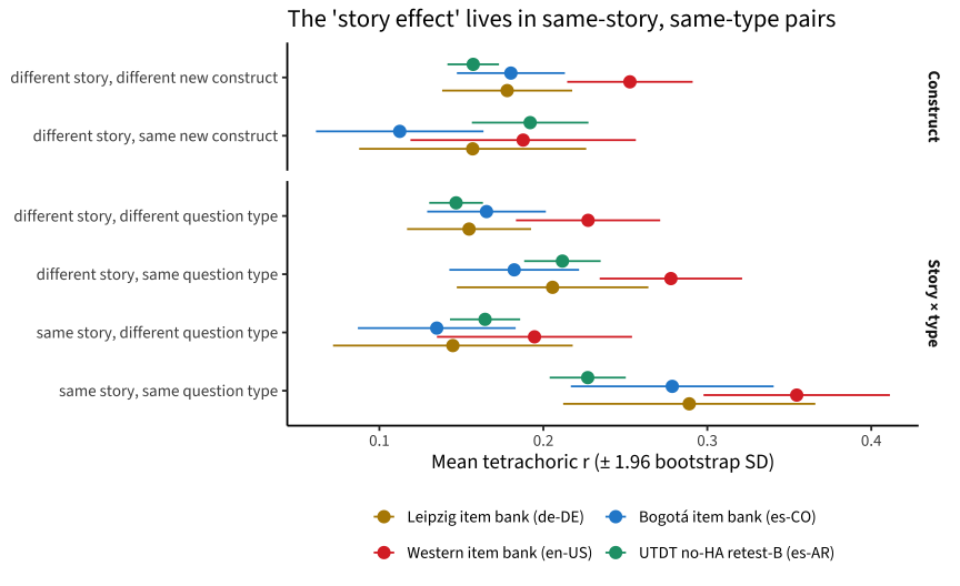
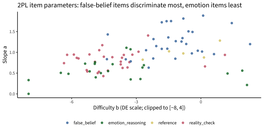
  • What organizes the items. Question type organizes item difficulty (R² .297, against .074 and .081 for the two story-construct schemes). Above the guessing floor, false-belief targets are more age-sensitive than controls (difference .14 [.04, .24] logits per year), so June’s “false-belief targets carry the age signal” survives on the chance-corrected scale; raw logit slopes do not separate them. The clustering of tetrachoric correlations by question type partly reflects shared difficulty: on IRT residuals the contrast shrinks to .006–.056, weak and uneven across samples.
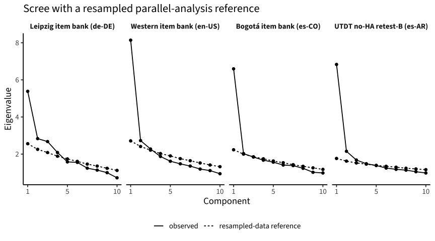
  • Dimensionality. A single score is defensible, most clearly outside Leipzig. The Leipzig form’s eigenvalue ratio is 1.90, as in June (on a partly different item set); the Western, Bogotá and es-AR forms are at 2.99–3.25. In the bifactor models ECV is .59–.73 (below the usual .70 in Leipzig and es-AR), and scores barely change (r = .955–.990). Story-level local dependence makes a unidimensional model overstate information by 13%–23%.
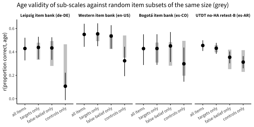
  • Controls. Keep them. They add reliability and cost almost no age validity. Their correlation with targets is .34 within dataset × form, lower than the pooled .48 that June’s method gives.
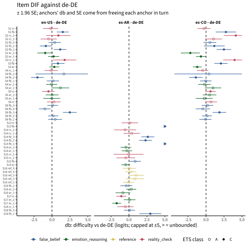
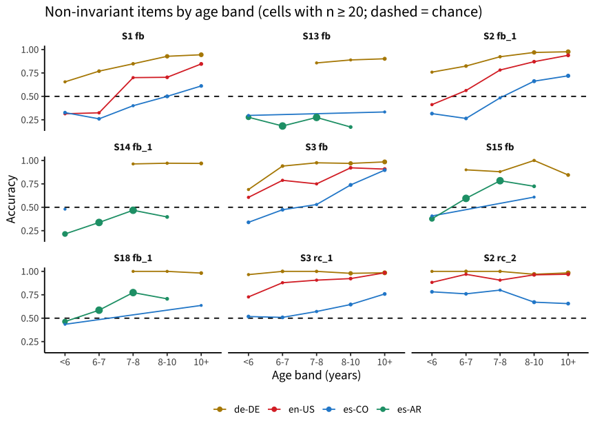
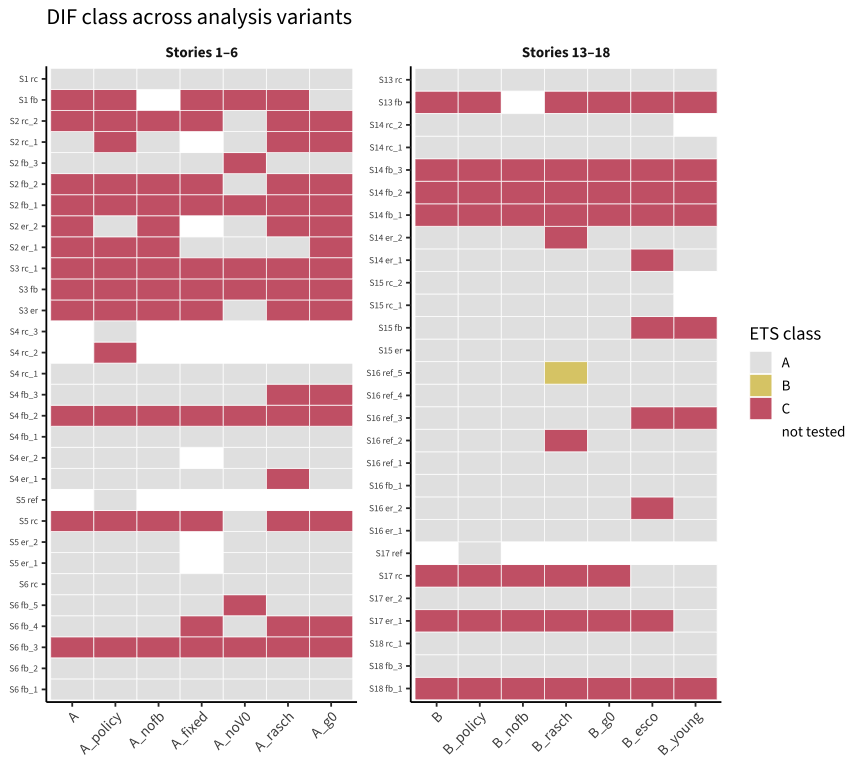
  • Cross-language invariance. In stories 1–6 (de/en-US/es-CO) the LR test rejects scalar invariance (χ²/df 7.2), but BIC does not favour non-invariance under the LEVANTE convention or the 2PL (Rasch dBIC 7, 2PL -68); it does with a guessing floor of 0 for below-chance items (dBIC 96). Stories 13–18 (de/es-AR) are non-invariant under both models (dBIC 168 and 87). Whether controls or targets carry more of the DIF depends on the model and the design, so June’s “controls dominate” is weakened, not simply overturned. False-belief items are non-invariant in both analyses, but language is confounded with prior exposure (most German children in stories 13–18 were on a repeat run), age and site. Two sites that share a language differ less (by BIC) and mostly on other items, and German children under 9 show the same false-belief DIF, so neither site nor age alone explains it. Partial scalar models fit, but only as a description.
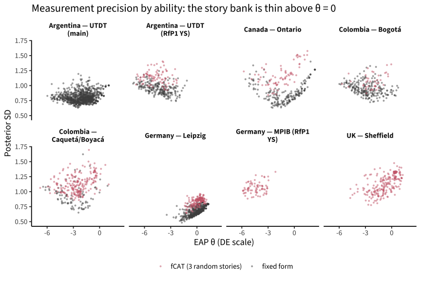
  • Reliability. Per administration, reliability is moderate: .56–.82 per dataset, pooling its fixed forms (single forms .36–.82), and .30–.65 for the deployed fCAT (3 random stories, median 4.4–5.6 minutes). Both are upper bounds. June’s “.92” was a model-implied value for a 58-item pool that no child takes; the same model’s reliability for what children answered is .554. In the same children, choosing the more informative story per block instead of a random one raises the reliability of a 3-story form by a median of .05 (up to .12). German alternate-form stability over 2–6 months is .50 [.40, .61].
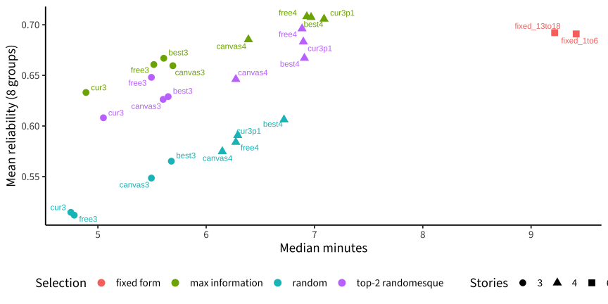
  • Block CAT (simulation). Choosing the most informative story within today’s three blocks raises mean reliability from .51 to .63 in the same time; adding a fourth, free story reaches .71 in about 7.1 median minutes, more than a fixed six-story form in less time. Select by information at the current estimate (not by discrimination), under the group’s prior; see Designing the block CAT.
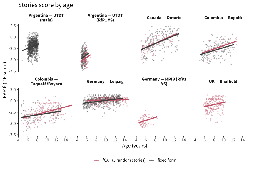
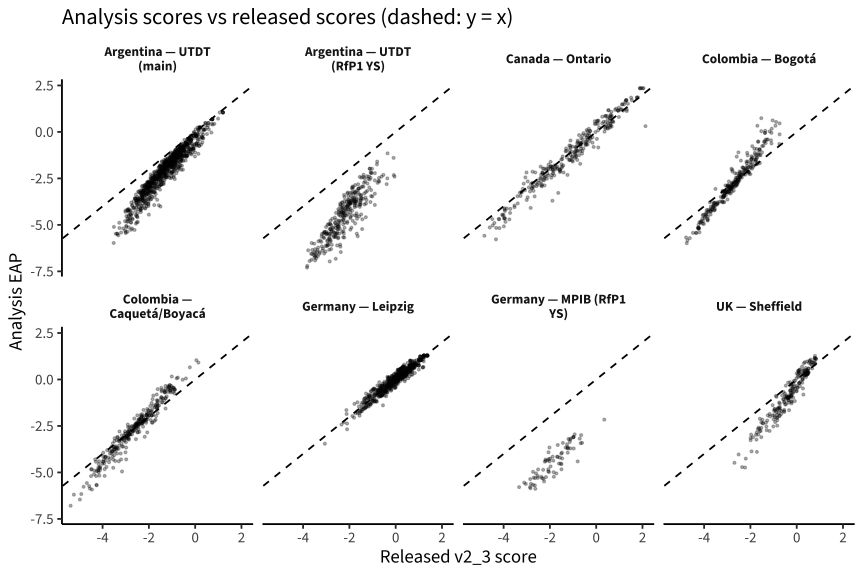
  • Scoring. The means and variances of low-scoring groups are weakly identified: they move with the integration grid, the latent density and the guessing convention, while scores within a group barely change. Datasets without their own group in v2_3 were scored under the German prior; with their own prior, their level drops by .5–2.5 logits.

Data and provenance

Code
prov <- attr(trials, "provenance")
prov$raw_sources |>
  left_join(prov$release_refs, by = "dataset") |>
  mutate(dataset = ds_label(dataset)) |>
  knitr::kable(caption = "Pinned raw datasets (read) and the latest processed releases (for reconciliation only)")
Pinned raw datasets (read) and the latest processed releases (for reconciliation only)
dataset raw_ref pulled_at release_ref
US — LangCog (downext) pilot_langcog_us_downex_raw:a6kb:v11_1 2026-09-24 15:08:24 pilot_langcog_us_downex:d3f2:v5_0
Germany — Leipzig pilot_mpieva_de_main_raw:6c0n:v16_15 2026-09-24 15:07:41 pilot_mpieva_de_main:8wjx:v7_2
Colombia — Bogotá pilot_uniandes_co_bogota_raw:3j4z:v17_0 2026-09-24 15:06:03 pilot_uniandes_co_bogota:d0c5:v5_1
Colombia — Caquetá/Boyacá pilot_uniandes_co_rural_raw:66d2:v16_0 2026-09-24 15:07:20 pilot_uniandes_co_rural:bxgv:v5_1
Canada — Ontario pilot_western_ca_main_raw:97mt:v16_12 2026-09-24 15:08:11 pilot_western_ca_main:bgcj:v5_1
rfp1_mpib_de_main rfp1_mpib_de_main_raw:0yye:v4_11 2026-09-24 15:05:30 rfp1_mpib_de_main:1s67:v3_1
Germany — MPIB (RfP1 YS) rfp1_mpib_intl_ys_raw:3r52:v6_0 2026-09-24 15:06:16 rfp1_mpib_intl_ys:cqyz:v2_1
UK — Sheffield rfp1_sheffield_gb_main_raw:5tmz:v3_25 2026-09-24 15:07:03 rfp1_sheffield_gb_main:3pzs:next
Argentina — UTDT (main) rfp1_utdt_ar_main_raw:3vkz:v4_13 2026-09-24 15:06:31 rfp1_utdt_ar_main:2b4m:v4_0
Argentina — UTDT (RfP1 YS) rfp1_utdt_intl_ys_raw:8cjy:v4_9 2026-09-24 15:07:55 rfp1_utdt_intl_ys:csvh:v4_0
  • Build. tasks/_build_stories_data.R ran process_trials() with levantemodels from the PR #27 branch (fix-tom-identity-corrections, commit 3dc148b, which sits directly on main bd24157). On 2026-09-24, git ls-remote gave bd24157 for origin/main (the same as the local main) and 3dc148b for refs/pull/27/head. Item identity metadata: levante_metadata_items:czjv:v3_18.
  • Run and trial rules. These are the production rules the latest releases were built with: no_data, task_bug (1.0.0-beta.19), incomplete, straightlining, duplicate (first run per user x task x variant x administration); trials: drop item_task NA or ‘ha’; drop rt_numeric > 60000; drop ‘fast’ message or rt_numeric < 300; then drop runs left with < 10 trials.
  • Reconciliation. Without PR #27 the rebuild reproduces the releases trial for trial (0 rebuilt trials missing from the releases, and 0 the other way round). For Sheffield the comparison is with its unreleased next draft of 2026-09-24 (:next in the table above), because its latest release (v3_1) predates the pinned raw data. The table below shows what PR #27 adds.
  • The fCAT is not adaptive. The theory-of-mind-item-bank-cat-test corpus (“fCAT”) shows one random story from each of 3 story groups. It has no item parameters and makes no θ updates. It is analysed here as a random 3-story form (fcat_random3).
Code
trials |>
  group_by(dataset, form, language) |>
  summarise(runs = n_distinct(run_id), children = n_distinct(user_id),
            trials = n(), median_age = median(age[!duplicated(run_id)], na.rm = TRUE),
            stories = story_ranges(story),
            first = as.Date(min(time_started)), last = as.Date(max(time_started)),
            .groups = "drop") |>
  mutate(dataset = ds_label(dataset)) |>
  knitr::kable(digits = 1, format.args = list(big.mark = ","),
               caption = "Included runs by dataset × form × language")
Included runs by dataset × form × language
dataset form language runs children trials median_age stories first last
US — LangCog (downext) item_bank en-US 7 7 207 3.9 1–6 2025-04-28 2025-05-12
Germany — Leipzig fcat_random3 de-DE 182 182 2,642 10.1 1–18 2026-08-26 2026-09-24
Germany — Leipzig item_bank de-DE 313 275 9,332 9.0 1–6 2024-09-18 2026-03-30
Germany — Leipzig no_ha de-DE 1 1 31 10.3 1–6 2026-08-20 2026-08-20
Germany — Leipzig retest_A de-DE 69 69 1,921 9.6 7–12 2025-04-07 2025-06-09
Germany — Leipzig retest_B de-DE 112 112 3,250 8.9 13–18 2025-04-05 2025-06-01
Colombia — Bogotá fcat_random3 es-CO 40 40 566 8.6 1–18 2026-08-26 2026-08-27
Colombia — Bogotá item_bank es-CO 229 229 6,132 8.4 1–6 2024-05-07 2024-06-14
Colombia — Caquetá/Boyacá co_retest_A es-CO 44 44 1,327 11.4 2, 7–12 2025-03-25 2025-11-05
Colombia — Caquetá/Boyacá co_retest_B es-CO 15 15 401 7.1 2, 13–18 2025-07-14 2025-11-05
Colombia — Caquetá/Boyacá fcat_random3 es-CO 216 216 3,180 9.6 1–18 2026-08-18 2026-08-31
Colombia — Caquetá/Boyacá item_bank es-CO 32 32 991 6.3 1–6 2024-10-29 2024-10-30
Canada — Ontario fcat_random3 en-US 76 76 1,124 7.2 1–18 2026-07-17 2026-09-24
Canada — Ontario item_bank en-US 201 196 6,206 8.5 1–6 2024-11-15 2026-04-22
rfp1_mpib_de_main fcat_random3 de-DE 7 7 108 4.7 1–11, 13–14, 16–17 2026-08-31 2026-09-24
rfp1_mpib_de_main no_ha de-DE 2 2 62 7.0 1–6 2026-08-10 2026-08-24
Germany — MPIB (RfP1 YS) fcat_random3 es-CO 75 75 1,129 5.7 1–18 2026-05-05 2026-05-22
UK — Sheffield fcat_random3 en-GB 216 216 3,191 7.7 1–18 2026-08-19 2026-09-24
Argentina — UTDT (main) no_ha_retest_B es-AR 943 943 28,214 7.0 13–18 2026-06-11 2026-09-24
Argentina — UTDT (RfP1 YS) co_retest_B es-CO 12 12 308 5.8 2, 13–18 2026-09-01 2026-09-16
Argentina — UTDT (RfP1 YS) fcat_random3 es-CO 86 86 1,247 5.8 1–18 2026-08-31 2026-09-21
Argentina — UTDT (RfP1 YS) no_ha_retest_B es-AR 217 217 6,436 5.3 13–18 2026-04-29 2026-06-29
Code
recon$per_dataset |>
  select(dataset, release_trials, stories_trials, added, relabelled,
         correct_differs, release_runs, stories_runs) |>
  mutate(dataset = ds_label(dataset)) |>
  knitr::kable(format.args = list(big.mark = ","),
               caption = "What PR #27 changes against the latest releases (trials and runs)")
What PR #27 changes against the latest releases (trials and runs)
dataset release_trials stories_trials added relabelled correct_differs release_runs stories_runs
US — LangCog (downext) 192 207 15 15 0 7 7
Germany — Leipzig 16,921 17,176 255 422 0 677 677
Colombia — Bogotá 6,146 6,698 552 222 0 267 269
Colombia — Caquetá/Boyacá 5,899 5,899 0 30 0 307 307
Canada — Ontario 6,770 7,330 560 746 0 277 277
rfp1_mpib_de_main 170 170 0 0 0 9 9
Germany — MPIB (RfP1 YS) 1,129 1,129 0 0 0 75 75
UK — Sheffield 3,191 3,191 0 0 0 216 216
Argentina — UTDT (main) 28,214 28,214 0 0 0 943 943
Argentina — UTDT (RfP1 YS) 7,991 7,991 0 0 0 315 315

Item-policy flags

The analyses drop the policy_exclude trials by default and analyse the spanish_fb_flag trials both with and without. Neither flag removes rows from the data file.

Code
trials |>
  filter(policy_exclude | spanish_fb_flag) |>
  mutate(flag = if_else(policy_exclude, policy_reason,
                        "Spanish reality_known false belief: analyse with and without")) |>
  group_by(flag, item = uid_label(story_uid), item_original) |>
  summarise(trials = n(), datasets = n_distinct(dataset),
            accuracy = mean(correct), chance = first(chance), .groups = "drop") |>
  arrange(flag, item) |>
  knitr::kable(digits = 3, format.args = list(big.mark = ","),
               caption = "Item-policy flags: trials, content code and accuracy")
Item-policy flags: trials, content code and accuracy
flag item item_original trials datasets accuracy chance
Spanish reality_known false belief: analyse with and without S1 fb 1c 327 4 0.431 0.50
Spanish reality_known false belief: analyse with and without S13 fb 13c 1,255 5 0.239 0.50
Spanish reality_known false belief: analyse with and without S7 fb 7c 118 4 0.356 0.50
reference_reference (stories 5/11/17): below chance in every language except German story 5 (at chance); negative item-rest r in every story S11 ref 11b 252 8 0.135 0.33
reference_reference (stories 5/11/17): below chance in every language except German story 5 (at chance); negative item-rest r in every story S17 ref 17b 1,452 9 0.066 0.33
reference_reference (stories 5/11/17): below chance in every language except German story 5 (at chance); negative item-rest r in every story S5 ref 5c 315 2 0.190 0.33
reference_reference (stories 5/11/17): below chance in every language except German story 5 (at chance); negative item-rest r in every story S5 ref 5c_new6 627 9 0.274 0.33
story-10 deception false belief 1: no discrimination (item-rest r CI spans 0 in every language) S10 fb_1 10d 257 8 0.669 0.50
story-2 reality check 1, first Bogota content (2e, May-June 2024): below chance; cause undetermined (inverted key, question identity or content) S2 rc_1 2e 229 1 0.087 0.50
story-4 reality checks 2/3 on image 4g (from 2024-10): rc_3 below chance in every language, rc_2 in de-DE and en-US (weak in en-GB, at chance in es-CO); the ‘yes’ key conflicts with the 4g image S4 rc_2 4g 622 9 0.328 0.50
story-4 reality checks 2/3 on image 4g (from 2024-10): rc_3 below chance in every language, rc_2 in de-DE and en-US (weak in en-GB, at chance in es-CO); the ‘yes’ key conflicts with the 4g image S4 rc_3 4g 621 9 0.188 0.50

Western’s empty item-bank runs

Code
wca_empty <- runs |>
  filter(dataset == "pilot_western_ca_main", variant_id == "Qx8XB8ZAFwP0RhhiEKw5",
         time_started >= as.POSIXct("2026-04-25", tz = "UTC"), n_trials_raw == 0)
wca_other <- runs |>
  filter(dataset == "pilot_western_ca_main", included,
         user_id %in% wca_empty$user_id)

174 Western runs on the item-bank variant (Qx8XB8ZAFwP0RhhiEKw5) between 2026-04-25 and 2026-08-31 logged no trials (36 with stop_reason = taskAbort). They are excluded as no_data. 18 of the 88 children involved have an included ToM run (at any time) in these data. According to the engineering team’s follow-up, no collected data were lost. The variant still loaded the item-bank corpus, whose hostile-attribution prompts are missing from the English item-bank translation, so the task failed its startup corpus check and aborted before the first trial. The children completed the other tasks. The failure was written up in an internal incident report on 12 July, logged by error monitoring on 19 and 28 August, and is related to core-tasks#437 (open since 8 April). The engineering team believes the variant has since been updated; the last run on it in these data started on 2026-08-31, which fits an update but does not prove one. Engineering plans a nightly check of open assignments that reference stale (unregistered) variants and, in the longer term, moving existing assignments to new variants when an old one is deprecated. For this chapter, these are missing administrations, not dropped data.

Item quality and the exclusion list

Item screen

Each story item was screened in each language with at least 30 responses: accuracy against chance (exact binomial tests) and item-rest correlation. The item-rest r is computed within dataset × form and then Fisher-pooled. The flag levels are poor (below chance without credible discrimination, or item-rest r reliably negative), below chance but discriminating, ceiling (≥ .95), weak (not above chance, or item-rest r with a 95% CI upper bound below .20) and ok.1

Code
res_items$flag_summary$by_language |>
  select(language, ok, ceiling, weak, `below chance, discriminating`, poor, `n < 30`) |>
  knitr::kable(caption = "Item × language cells by flag (n ≥ 30 to be flagged)")
Item × language cells by flag (n ≥ 30 to be flagged)
language ok ceiling weak below chance, discriminating poor n < 30
de-DE 47 32 7 0 5 0
en-GB 56 15 9 0 3 6
en-US 27 0 1 0 3 58
es-AR 18 2 7 1 2 0
es-CO 67 0 17 1 7 0
Code
il <- res_items$items_lang |>
  filter(flag != "n < 30") |>
  mutate(label = uid_label(story_uid),
         label = paste0(label, case_when(content == "other content" ~ " [other content]",
                                         str_detect(content, "4g") ~ " [4g]",
                                         str_detect(content, "2e") ~ " [2e]",
                                         TRUE ~ "")),
         label = fct_reorder(label, -story),
         question_type = factor(question_type, qtype_levels),
         language = factor(language, lang_levels),
         flag = fct_drop(flag))
ggplot(il, aes(x = accuracy - chance, y = label, colour = language, shape = flag)) +
  geom_vline(xintercept = 0, linetype = "dashed") +
  geom_point(size = 2, alpha = .8) +
  facet_wrap(vars(question_type), scales = "free_y", ncol = 2) +
  scale_colour_manual(values = lang_pal, name = NULL) +
  scale_shape_manual(values = c(ok = 16, ceiling = 17, weak = 1,
                                `below chance, discriminating` = 4, poor = 8), name = NULL) +
  labs(x = "Accuracy minus chance", y = NULL,
       title = "Item accuracy above chance, by language",
       subtitle = "Cells with n ≥ 30; [4g], [2e] and [other content] split the policy-flagged content from the rest") +
  theme(legend.position = "bottom", legend.box = "vertical",
        axis.text.y = element_text(size = 7))
Figure 28.1
Code
res_items$flag_summary$poor_not_policy |>
  transmute(item = uid_label(story_uid), language, n, accuracy, chance,
            p_below = fp(p_below), r_ir, r_ir_lo, flag, datasets) |>
  knitr::kable(digits = 3, caption = "Below-chance cells outside the policy flags")
Below-chance cells outside the policy flags
item language n accuracy chance p_below r_ir r_ir_lo flag datasets
S1 fb es-CO 327 0.431 0.5 0.0074 0.289 0.182 below chance, discriminating pilot_uniandes_co_bogota, pilot_uniandes_co_rural, rfp1_mpib_intl_ys, rfp1_utdt_intl_ys
S7 fb es-CO 118 0.356 0.5 0.0011 0.189 -0.027 poor pilot_uniandes_co_bogota, pilot_uniandes_co_rural, rfp1_mpib_intl_ys, rfp1_utdt_intl_ys
S13 fb es-AR 1158 0.235 0.5 <1e-04 0.016 -0.042 poor rfp1_utdt_ar_main, rfp1_utdt_intl_ys
S13 fb es-CO 97 0.289 0.5 <1e-04 0.056 -0.269 poor pilot_uniandes_co_bogota, pilot_uniandes_co_rural, rfp1_mpib_intl_ys, rfp1_utdt_intl_ys
S14 fb_1 es-AR 1159 0.368 0.5 <1e-04 0.184 0.128 below chance, discriminating rfp1_utdt_ar_main, rfp1_utdt_intl_ys
Code
ia <- function(uid, cont = "all", col = accuracy)
  pick(res_items$items_all, {{ col }}, story_uid == uid, content == cont)
il_acc <- function(uid, lang, col = accuracy)
  pick(res_items$items_lang, {{ col }}, story_uid == uid, language == lang, content == "all")
k$s14_ar    <- il_acc("tom_story14_moral_reasoning_false_belief_1", "es-AR")
k$s14_ar_n  <- il_acc("tom_story14_moral_reasoning_false_belief_1", "es-AR", n)
k$s14_ar_r  <- il_acc("tom_story14_moral_reasoning_false_belief_1", "es-AR", r_ir)
k$s14_ar_lo <- il_acc("tom_story14_moral_reasoning_false_belief_1", "es-AR", r_ir_lo)
k$s14_ar_hi <- il_acc("tom_story14_moral_reasoning_false_belief_1", "es-AR", r_ir_hi)
k$s14_ar_age <- il_acc("tom_story14_moral_reasoning_false_belief_1", "es-AR", median_age)
k$s14_de    <- il_acc("tom_story14_moral_reasoning_false_belief_1", "de-DE")
rk_band <- \(uid, lang, band) pick(res_items$rk_fb_age, accuracy, story_uid == uid, language == lang,
                                   age_band == band)
rk_am <- res_items$rk_fb_age_matched

What the screen shows:

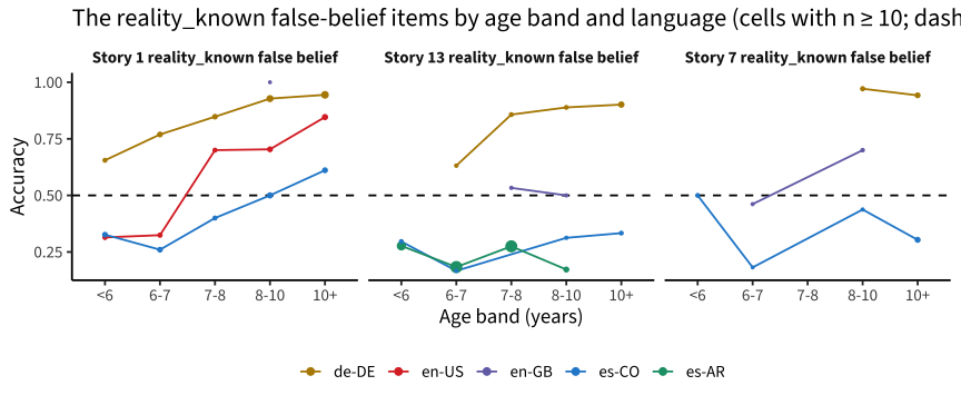
  • Outside the policy flags, the below-chance cells are Spanish false-belief items, above all the reality_known question (“where will X look first?”) of stories 1, 7 and 13. They are not alike. Story 1 in es-CO is below chance but discriminates (item-rest r .29 [.18, .39]), the pattern of children who answer with the object’s real location. Story 7 in es-CO has a similar r (.19 [-.03, .39], n = 118) and is flagged poor only because its interval reaches 0. Story 13 in es-AR carries no information: .235 correct, item-rest r .016.
  • The failure is not specific to Spanish. Young en-US children are also below chance on story 1 (.31 under 6 and .32 at 6–7 years), and story 13 is at chance in en-GB (.47, n = 36). The items “work” only in the older German samples. Compared at the same age, though, Spanish-speaking children still answer them less often correctly (table below): the Spanish gap is 1.6–2.6 logits. Age, language, site and sample are confounded, and nobody has checked the translation files yet.
Code
res_items$rk_fb_age |>
  filter(n >= 10) |>
  mutate(item = paste0("Story ", story, " reality_known false belief"),
         language = factor(language, lang_levels)) |>
  ggplot(aes(age_band, accuracy, colour = language, group = language)) +
  geom_hline(aes(yintercept = chance), linetype = "dashed") +
  geom_line() + geom_point(aes(size = n)) +
  facet_wrap(vars(item), nrow = 1) +
  scale_colour_manual(values = lang_pal, name = NULL) +
  scale_size_area(max_size = 3, guide = "none") +
  labs(x = "Age band (years)", y = "Accuracy",
       title = "The reality_known false-belief items by age band and language (cells with n ≥ 10; dashed = chance)") +
  theme(legend.position = "bottom")
rk_am |>
  transmute(item = uid_label(story_uid), ages = paste0(n2(age_lo, 1), "–", n2(age_hi, 1)),
            n_es, n_other, other_languages, spanish_logit = es_logit, lo = es_lo, hi = es_hi,
            acc_at_7_other, acc_at_7_es) |>
  knitr::kable(digits = 2, caption = "Age-matched comparison: glm(correct ~ age + Spanish) on the ages both groups cover (the intersection of each group's 5th–95th age percentiles)")
item ages n_es n_other other_languages spanish_logit lo hi acc_at_7_other acc_at_7_es
S1 fb 5.5–11.7 225 493 de-DE, en-GB, en-US -1.64 -2.00 -1.28 0.70 0.31
S13 fb 6.1–8.1 938 76 de-DE, en-GB, en-US -1.87 -2.37 -1.37 0.65 0.22
S7 fb 6.1–12.6 83 132 de-DE, en-GB, en-US -2.56 -3.28 -1.83 0.74 0.18
Figure 28.2: Age-matched comparison: glm(correct ~ age + Spanish) on the ages both groups cover (the intersection of each group’s 5th–95th age percentiles)
Figure 28.3
  • The problem reaches beyond stories 1/7/13. Story 14’s moral-reasoning false belief (“where will he look first for his soccer ball?”) is below chance in es-AR (.368, n = 1,159; de-DE .933), yet its item-rest r is positive (.184 [.128, .239]). That pattern fits young children (median age 6.8) who answer with the real location, not a broken key. Age and language are confounded here: the es-AR samples are the youngest.
  • The weakest items outside the policy flags are yes/no “Is [sibling] mad at [sibling]?” questions in the parallel deception stories 4 and 16. They sit at or near chance everywhere. Two other targets barely discriminate, and story 10’s deception false belief 1 does not discriminate at all (it is now policy-excluded; see the verdicts):
Code
weak_uids <- c("tom_story4_deception_false_belief_3", "tom_story16_deception_reference_2",
               "tom_story16_deception_reference_5", "tom_story10_deception_false_belief_1",
               "tom_story17_reference_emotion_reasoning_1")
res_items$items_all |>
  filter(story_uid %in% weak_uids, content == "all") |>
  transmute(item = uid_label(story_uid), prompt, n, accuracy, chance,
            r_ir, r_ir_lo, r_ir_hi, lang_weak) |>
  knitr::kable(digits = 3, caption = "Candidates for item revision (not proposed exclusions)")
Candidates for item revision (not proposed exclusions)
item prompt n accuracy chance r_ir r_ir_lo r_ir_hi lang_weak
S4 fb_3 Is Joshua mad at Isabel? 939 0.486 0.50 0.124 0.058 0.189 de-DE, en-GB, en-US, es-CO
S10 fb_1 Is Teacher Sarah lying? 257 0.669 0.50 -0.035 -0.171 0.102 de-DE, en-GB
S16 ref_2 Is Sophie mad at James? 1409 0.515 0.50 0.135 0.082 0.187 en-GB, es-AR, es-CO
S16 ref_5 Is Sophie mad at James now? 1401 0.598 0.50 0.083 0.030 0.137 en-GB, es-AR, es-CO
S17 er_1 Mom looks in the wrong stack of books and can’t find the book that she wanted. How do you think Mom feels about not finding the book she wanted? 1451 0.689 0.25 -0.004 -0.057 0.049 de-DE, es-AR

content splits the policy-flagged 4g and 2e content from the rest. Flagged languages are listed by flag level.

Code
res_items$items_all |>
  arrange(story, question_type) |>
  transmute(item = uid_label(story_uid), content, question_type, prompt, n,
            accuracy, chance, r_ir, r_ir_lo, r_ir_hi,
            lang_poor, lang_below_disc, lang_weak, lang_ceiling) |>
  knitr::kable(digits = 3)
item content question_type prompt n accuracy chance r_ir r_ir_lo r_ir_hi lang_poor lang_below_disc lang_weak lang_ceiling
S1 fb all false_belief Where will Madison look for her book first? 924 0.658 0.50 0.359 0.299 0.416 es-CO
S1 rc all reality_check And where is her book really? 925 0.912 0.50 0.250 0.184 0.313 de-DE
S2 er_1 all emotion_reasoning How do you think Hannah feels about Ethan reaching for that book? 963 0.841 0.25 0.199 0.135 0.262
S2 er_2 all emotion_reasoning How do you think Hannah would feel if she had not seen Ethan reaching for the book? 639 0.397 0.25 0.178 0.098 0.256
S2 fb_1 all false_belief Now, when Ethan comes in from outside, where will he look first for his book? 972 0.725 0.50 0.334 0.275 0.391 es-CO
S2 fb_2 all false_belief Is Ethan being mean and naughty for taking Hannah’s book? 952 0.686 0.50 0.220 0.156 0.282 es-CO
S2 fb_3 all false_belief Should Ethan get in trouble with the teacher for taking Hannah’s book? 951 0.740 0.50 0.225 0.161 0.287
S2 rc_1 other content reality_check Can you help Hannah find her book? Is it on the shelf or under the coats? 719 0.915 0.50 0.210 0.134 0.284 de-DE
S2 rc_1 policy-flagged (2e) reality_check Can you help Hannah find her book? Is it on the shelf or under the coats? 229 0.087 0.50 -0.112 -0.239 0.018 es-CO
S2 rc_2 all reality_check Can you help Ethan find his book? Is it on the shelf or under the coats? 943 0.876 0.50 0.079 0.012 0.145 es-CO de-DE, en-GB
S3 er all emotion_reasoning Look, Isabel and Ivan found Joshua, and won the game! How do you think Isabel feels about winning the game? 939 0.728 0.25 0.169 0.104 0.233
S3 fb all false_belief When Isabel and Ivan see this clue, where will they look first for Joshua? 946 0.775 0.50 0.309 0.248 0.369
S3 rc_1 all reality_check What did Joshua mean to draw? 948 0.829 0.50 0.231 0.166 0.293 de-DE
S3 rc_2 all reality_check Can you help them find where Joshua really is? 946 0.961 0.50 0.139 0.071 0.205 de-DE, en-GB
S4 er_1 all emotion_reasoning How does Joshua feel about losing his truck? 941 0.892 0.25 0.213 0.149 0.275 de-DE
S4 er_2 all emotion_reasoning How would Joshua feel if he found his truck? 623 0.769 0.25 0.324 0.248 0.396
S4 fb_1 all false_belief Is it fair that Mother is mad at Joshua for losing his truck? 938 0.810 0.50 0.194 0.129 0.257 es-CO
S4 fb_2 all false_belief Is Mother mad at Isabel? 940 0.645 0.50 0.369 0.311 0.425
S4 fb_3 all false_belief Is Joshua mad at Isabel? 939 0.486 0.50 0.124 0.058 0.189 de-DE, en-GB, en-US, es-CO
S4 rc_1 all reality_check Is Mother mad at Joshua now? 937 0.860 0.50 0.279 0.217 0.339
S4 rc_2 other content reality_check Is Mother mad at Isabel now? 315 0.635 0.50 0.284 0.178 0.383
S4 rc_2 policy-flagged (4g) reality_check Is Mother mad at Isabel now? 622 0.328 0.50 -0.088 -0.169 -0.005 de-DE, en-US en-GB, es-CO
S4 rc_3 other content reality_check Is Joshua mad at Isabel now? 316 0.566 0.50 0.225 0.117 0.328 de-DE
S4 rc_3 policy-flagged (4g) reality_check Is Joshua mad at Isabel now? 621 0.188 0.50 -0.117 -0.198 -0.034 de-DE, en-GB, en-US, es-CO
S5 er_1 all emotion_reasoning How does Katie feel about not getting the cup she wanted? 627 0.925 0.25 0.214 0.130 0.294 de-DE
S5 er_2 all emotion_reasoning How would Katie feel if she had received the cup she wanted? 627 0.841 0.25 0.385 0.313 0.453
S5 rc all reality_check Which cup does Katie want? 941 0.830 0.33 0.284 0.221 0.346
S5 ref all reference Which cup will Dad give Katie? 942 0.246 0.33 -0.165 -0.228 -0.100 de-DE, en-US, es-CO
S6 fb_1 all false_belief Does Sam know that Maria bought some socks? 952 0.867 0.50 0.285 0.224 0.344 de-DE
S6 fb_2 all false_belief What does Sam think they are selling at the shop? 951 0.578 0.33 0.394 0.337 0.448
S6 fb_3 all false_belief What does Maria tell dad? 950 0.680 0.50 0.338 0.278 0.395 es-CO
S6 fb_4 all false_belief What does Maria tell dad? 948 0.467 0.33 0.238 0.175 0.299 es-CO
S6 fb_5 all false_belief What does Sam think they are selling at the shop? 950 0.535 0.33 0.273 0.211 0.332 es-CO
S6 rc all reality_check Does Maria know that they are selling shoes in the shop? 951 0.845 0.50 0.268 0.206 0.329 de-DE
S7 fb all false_belief Where will Diana look for her toy? 273 0.619 0.50 0.240 0.110 0.363 es-CO en-GB
S7 rc all reality_check And where is her toy really? 273 0.930 0.50 0.083 -0.052 0.215 es-CO de-DE, en-GB
S8 er_1 all emotion_reasoning How do you think Mike feels about Allie reaching for that pencil? 251 0.904 0.25 0.112 -0.028 0.247 de-DE
S8 er_2 all emotion_reasoning How do you think Mike would feel if he had not seen Allie reaching for the pencil? 249 0.502 0.25 0.089 -0.052 0.226 de-DE, en-GB
S8 fb_1 all false_belief Now, when Allie comes in from outside, where will she look first for her pencil? 251 0.817 0.50 0.224 0.088 0.352 de-DE, en-GB
S8 fb_2 all false_belief Is Allie being mean and naughty for taking Mike’s pencil? 251 0.793 0.50 0.127 -0.013 0.261 de-DE
S8 fb_3 all false_belief Should Allie get in trouble with the teacher for taking Mike’s pencil? 251 0.777 0.50 0.241 0.094 0.378
S8 rc_1 all reality_check Can you help Mike find his pencil? Is it on top of the shelf or behind the backpack shelf? 251 0.896 0.50 0.200 0.063 0.330 de-DE
S8 rc_2 all reality_check Can you help Allie find her pencil? Is it on top of the shelf or behind the backpack shelf? 250 0.968 0.50 0.351 0.170 0.509 de-DE, en-GB
S9 er all emotion_reasoning Look, Mom realized her mistake and gave Mark the book he really wanted! How do you think Mark feels about getting the book he wanted? 243 0.864 0.25 0.245 0.107 0.373 en-GB
S9 fb all false_belief When Mom sees the picture, what book will she give Mark? 243 0.798 0.50 0.119 -0.032 0.265 de-DE
S9 rc_1 all reality_check What did Mark mean to draw? 245 0.951 0.50 0.302 0.118 0.466 de-DE, en-GB
S9 rc_2 all reality_check What book does Mark really want? 246 0.935 0.50 0.147 -0.002 0.290 de-DE, en-GB
S10 er_1 all emotion_reasoning How does Megan feel about being the only child without a storybook? 258 0.911 0.25 0.111 -0.041 0.258
S10 er_2 all emotion_reasoning How would Megan feel if she received a book? 257 0.887 0.25 0.134 -0.003 0.266 de-DE
S10 fb_1 all false_belief Is Teacher Sarah lying? 257 0.669 0.50 -0.035 -0.171 0.102 de-DE, en-GB
S10 rc_1 all reality_check Is Brian lying? 258 0.888 0.50 0.081 -0.056 0.215 es-CO en-GB
S10 rc_2 all reality_check Is there still a storybook left, that isn’t being used right now? 258 0.899 0.50 0.279 0.149 0.401
S10 rc_3 all reality_check Is there still a storybook left, that isn’t being used right now? 258 0.907 0.50 0.163 0.027 0.293
S11 er_1 all emotion_reasoning Josh wanted the baseball but mom gave him the soccer ball! How do you think Josh feels about receiving the wrong toy? 252 0.929 0.25 0.226 0.094 0.351
S11 er_2 all emotion_reasoning How do you think Josh would feel if he had received the correct toy? 250 0.848 0.25 0.139 0.003 0.270
S11 rc all reality_check Which ball does Josh want? 252 0.829 0.33 0.213 0.080 0.339 en-GB
S11 ref all reference Which ball will mom get for Josh? 252 0.135 0.33 -0.198 -0.325 -0.064 de-DE, en-GB, es-CO
S12 fb_1 all false_belief Which toy does Dad think Emma wants to bring to school? 248 0.718 0.50 0.212 0.076 0.339 es-CO
S12 fb_2 all false_belief Does Emma know that Dad packed the blue ball? 249 0.924 0.50 0.236 0.072 0.387 de-DE, en-GB
S12 fb_3 all false_belief Which ball does Emma think Dad packed? 249 0.747 0.33 0.221 0.086 0.348
S12 rc_1 all reality_check What toy does Emma want? 248 0.855 0.33 0.124 -0.014 0.258
S12 rc_2 all reality_check What toy did Dad pack for Emma? 248 0.923 0.33 0.056 -0.111 0.221 de-DE
S13 fb all false_belief Where will Gabriel look for his pencil? 1451 0.308 0.50 0.053 0.000 0.106 es-AR, es-CO en-GB
S13 rc all reality_check And where is his pencil really? 1450 0.899 0.50 0.145 0.092 0.196 es-AR de-DE
S14 er_1 all emotion_reasoning How do you think Anna feels about Bobby reaching for that soccer ball? 1449 0.791 0.25 0.151 0.099 0.203
S14 er_2 all emotion_reasoning How do you think Anna would feel if she had not seen Bobby reaching for the soccer ball? 1447 0.387 0.25 0.149 0.097 0.201 en-GB
S14 fb_1 all false_belief Now, when Bobby comes in from outside, where will he look first for his soccer ball? 1448 0.452 0.50 0.211 0.160 0.261 es-AR es-CO
S14 fb_2 all false_belief Is Bobby being mean and naughty for taking Anna’s soccer ball? 1447 0.644 0.50 0.168 0.116 0.219
S14 fb_3 all false_belief Should Bobby get in trouble with their mom for taking Anna’s soccer ball? 1447 0.601 0.50 0.144 0.092 0.195 es-AR
S14 rc_1 all reality_check Can you help Anna find her soccer ball? Is it on the table or on the floor? 1449 0.876 0.50 0.136 0.084 0.188 de-DE
S14 rc_2 all reality_check Can you help Bobby find his soccer ball? Is it on the table or on the floor? 1449 0.956 0.50 0.187 0.135 0.238 de-DE, en-GB, es-AR
S15 er all emotion_reasoning Look, Alex and Beth found Johnny, and won the game! How do you think Alex and Beth feel about winning the game? 1445 0.662 0.25 0.142 0.090 0.194 es-AR
S15 fb all false_belief When Alex and Beth see this clue, where will they look first for Johnny? Behind the flower bush or behind the rock? 1444 0.652 0.50 0.334 0.286 0.380 de-DE, es-CO
S15 rc_1 all reality_check What did Johnny mean to draw? 1447 0.930 0.50 0.239 0.188 0.288 de-DE
S15 rc_2 all reality_check Can you help them find where Johnny really is? 1447 0.964 0.50 0.202 0.147 0.255 de-DE, en-GB, es-AR
S16 er_1 all emotion_reasoning How does Sophie feel about losing her shoe? 1414 0.906 0.25 0.130 0.076 0.182 es-AR de-DE
S16 er_2 all emotion_reasoning How would Sophie feel if she found her shoe? 1411 0.669 0.25 0.226 0.175 0.277
S16 fb_1 all false_belief Is it fair that Dad is mad at Sophie for losing her shoe? 1410 0.819 0.50 0.247 0.196 0.297
S16 ref_1 all reference Is Dad mad at James? 1409 0.637 0.50 0.239 0.187 0.289
S16 ref_2 all reference Is Sophie mad at James? 1409 0.515 0.50 0.135 0.082 0.187 en-GB, es-AR, es-CO
S16 ref_3 all reference Is Dad mad at Sophie now? 1402 0.787 0.50 0.156 0.103 0.209 de-DE
S16 ref_4 all reference Is Dad mad at James now? 1400 0.696 0.50 0.202 0.150 0.253
S16 ref_5 all reference Is Sophie mad at James now? 1401 0.598 0.50 0.083 0.030 0.137 en-GB, es-AR, es-CO
S17 er_1 all emotion_reasoning Mom looks in the wrong stack of books and can’t find the book that she wanted. How do you think Mom feels about not finding the book she wanted? 1451 0.689 0.25 -0.004 -0.057 0.049 de-DE, es-AR
S17 er_2 all emotion_reasoning How do you think Mom would feel if she could find the book she wanted? 1446 0.770 0.25 0.378 0.332 0.422 de-DE
S17 rc all reality_check Which stack of books was Mika talking about? 1451 0.815 0.33 0.186 0.134 0.236
S17 ref all reference Which stack of books will mom look in? 1452 0.066 0.33 -0.084 -0.137 -0.032 de-DE, en-GB, es-AR, es-CO
S18 fb_1 all false_belief Which toy does Kat think George wants from the toy shop? 1414 0.669 0.50 0.307 0.257 0.355 es-CO de-DE
S18 fb_2 all false_belief Does George know that Kat bought a storybook? 1409 0.903 0.50 0.327 0.276 0.376 de-DE, en-GB
S18 fb_3 all false_belief What does George think Kat bought at the toy shop? 1408 0.692 0.33 0.348 0.300 0.395
S18 rc_1 all reality_check What toy does George want? 1402 0.887 0.33 0.320 0.270 0.368 de-DE
S18 rc_2 all reality_check What toy did Kat buy for George? 1398 0.926 0.33 0.245 0.190 0.297 de-DE, en-GB
Code
res_items$items_cell |>
  filter(flag %in% c("poor", "below chance, discriminating")) |>
  arrange(story, dataset) |>
  transmute(item = uid_label(story_uid), content, dataset, form, language, n,
            accuracy, chance, median_age, r_ir, flag) |>
  knitr::kable(digits = 3)
item content dataset form language n accuracy chance median_age r_ir flag
S2 rc_1 policy-flagged (2e) pilot_uniandes_co_bogota item_bank es-CO 229 0.087 0.50 8.40 -0.112 poor
S2 rc_2 all pilot_uniandes_co_bogota item_bank es-CO 229 0.659 0.50 8.40 -0.190 poor
S2 fb_1 all pilot_uniandes_co_rural item_bank es-CO 32 0.219 0.50 6.35 -0.127 poor
S3 fb all pilot_uniandes_co_rural item_bank es-CO 32 0.250 0.50 6.35 -0.045 poor
S4 rc_2 policy-flagged (4g) pilot_mpieva_de_main item_bank de-DE 224 0.254 0.50 8.55 -0.220 poor
S4 rc_3 policy-flagged (4g) pilot_mpieva_de_main fcat_random3 de-DE 32 0.250 0.50 10.10 -0.253 poor
S4 rc_3 policy-flagged (4g) pilot_mpieva_de_main item_bank de-DE 224 0.143 0.50 8.55 -0.032 poor
S4 rc_3 policy-flagged (4g) pilot_uniandes_co_rural fcat_random3 es-CO 39 0.179 0.50 10.10 -0.042 poor
S4 rc_2 policy-flagged (4g) pilot_western_ca_main item_bank en-US 200 0.310 0.50 8.50 0.006 poor
S4 rc_3 policy-flagged (4g) pilot_western_ca_main item_bank en-US 199 0.161 0.50 8.50 -0.156 poor
S4 rc_3 policy-flagged (4g) rfp1_sheffield_gb_main fcat_random3 en-GB 30 0.200 0.50 8.00 -0.130 poor
S5 ref all pilot_mpieva_de_main item_bank de-DE 313 0.319 0.33 9.00 -0.161 poor
S5 ref all pilot_uniandes_co_bogota item_bank es-CO 226 0.195 0.33 8.40 -0.198 poor
S5 ref all pilot_uniandes_co_rural fcat_random3 es-CO 39 0.179 0.33 10.20 -0.317 poor
S5 ref all pilot_western_ca_main item_bank en-US 200 0.245 0.33 8.50 -0.107 poor
S6 fb_2 all pilot_uniandes_co_rural item_bank es-CO 32 0.062 0.33 6.35 -0.002 poor
S11 ref all pilot_mpieva_de_main retest_A de-DE 69 0.159 0.33 9.60 -0.102 poor
S11 ref all pilot_uniandes_co_rural fcat_random3 es-CO 39 0.051 0.33 9.30 -0.019 poor
S11 ref all rfp1_sheffield_gb_main fcat_random3 en-GB 43 0.047 0.33 7.60 -0.441 poor
S13 fb all pilot_uniandes_co_rural fcat_random3 es-CO 38 0.237 0.50 10.80 0.056 poor
S13 fb all rfp1_utdt_ar_main no_ha_retest_B es-AR 943 0.228 0.50 7.00 0.071 below chance, discriminating
S13 fb all rfp1_utdt_intl_ys no_ha_retest_B es-AR 215 0.265 0.50 5.30 -0.226 poor
S14 fb_1 all rfp1_utdt_ar_main no_ha_retest_B es-AR 943 0.403 0.50 7.00 0.217 below chance, discriminating
S14 fb_1 all rfp1_utdt_intl_ys no_ha_retest_B es-AR 216 0.213 0.50 5.30 0.036 poor
S15 fb all rfp1_utdt_intl_ys no_ha_retest_B es-AR 217 0.378 0.50 5.30 0.271 below chance, discriminating
S17 ref all pilot_mpieva_de_main fcat_random3 de-DE 39 0.128 0.33 10.10 0.025 poor
S17 ref all pilot_mpieva_de_main retest_B de-DE 108 0.111 0.33 8.90 -0.214 poor
S17 ref all pilot_uniandes_co_rural fcat_random3 es-CO 35 0.057 0.33 9.10 -0.017 poor
S17 ref all rfp1_sheffield_gb_main fcat_random3 en-GB 40 0.075 0.33 7.90 -0.368 poor
S17 ref all rfp1_utdt_ar_main no_ha_retest_B es-AR 938 0.046 0.33 7.00 -0.072 poor
S17 ref all rfp1_utdt_intl_ys no_ha_retest_B es-AR 215 0.121 0.33 5.30 -0.038 poor

Do higher scorers do better?

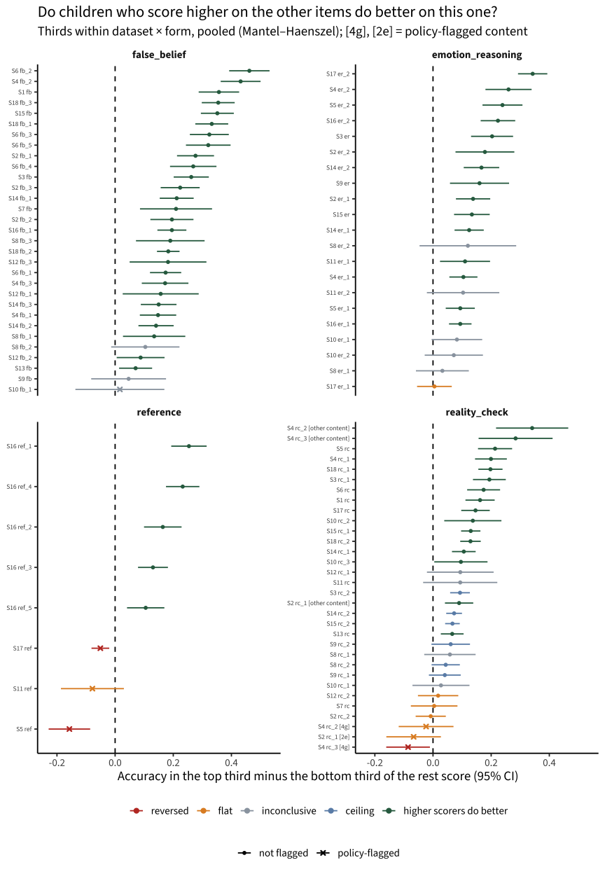
The item screen asks whether an item correlates with the rest of the test. A more direct check of what an item should do is whether children who do better on their other items also do better on this one. For each item, the responses in each dataset × form cell with at least 30 of them are split into thirds by the rest score used above (proportion correct on the run’s other non-policy items; ties broken at random). The accuracy difference between the top and the bottom third (the gain) is pooled over cells with Mantel–Haenszel weights and the Sato variance, so each site and form is compared only with itself. An item is reversed if the 95% CI of its gain lies below 0, flat if the CI includes 0 but rules out a gain of .10 or more, inconclusive if it includes both, at ceiling if accuracy is at least .95, and otherwise higher scorers do better. Items and item × language cells are classified from 90 responses.2 The screen is tasks/_stories_fits_monotonicity.R.

Code
mono_n <- \(cls) sum(res_mono$mono_all$mono == cls)
mono_row <- \(uid, col, cont = "all") pick(res_mono$mono_all, {{ col }}, story_uid == uid, content == cont)
mono_lang_row <- \(uid, lang, col) pick(res_mono$mono_lang, {{ col }}, story_uid == uid, content == "all",
                                        language == lang)
gain_ci <- \(d, lo, hi) paste0(n2(d), " [", n2(lo), ", ", n2(hi), "]")
er17 <- "tom_story17_reference_emotion_reasoning_1"
er17_share <- \(lg, th, emo) pick(res_mono$er17, share, lang == lg, third == th, emotion == emo)
s2v <- \(prt, col) pick(res_mono$s2rc2, {{ col }}, part == prt)
k$mono_policy_hit <- res_mono$mono_all |>
  filter(policy, mono %in% c("reversed", "flat")) |> nrow()
Code
res_mono$mono_all |>
  mutate(label = paste0(uid_label(story_uid),
                        case_when(str_detect(content, "4g") ~ " [4g]", str_detect(content, "2e") ~ " [2e]",
                                  content == "other content" ~ " [other content]", TRUE ~ "")),
         label = fct_reorder(label, diff),
         question_type = factor(question_type, qtype_levels),
         policy = if_else(policy, "policy-flagged", "not flagged")) |>
  ggplot(aes(x = diff, y = label, colour = mono, shape = policy)) +
  geom_vline(xintercept = 0, linetype = "dashed") +
  geom_pointrange(aes(xmin = diff_lo, xmax = diff_hi), size = .3) +
  facet_wrap(vars(question_type), scales = "free_y", ncol = 2) +
  scale_colour_manual(values = c(reversed = "#c0392b", flat = "#e08e2b", inconclusive = "#9aa3ae",
                                 ceiling = "#6b8fb5", `higher scorers do better` = "#2e6b4f"), name = NULL) +
  scale_shape_manual(values = c(`policy-flagged` = 4, `not flagged` = 16), name = NULL) +
  labs(x = "Accuracy in the top third minus the bottom third of the rest score (95% CI)", y = NULL,
       title = "Do children who score higher on the other items do better on this one?",
       subtitle = "Thirds within dataset × form, pooled (Mantel–Haenszel); [4g], [2e] = policy-flagged content") +
  theme(legend.position = "bottom", legend.box = "vertical", axis.text.y = element_text(size = 7))
Figure 28.4
  • Of the 92 item × content rows, 64 pass, 6 are at ceiling, 12 are inconclusive, 7 are flat and 3 are reversed.
  • The screen finds the existing exclusions on its own. The reversed rows are the reference questions of stories 5 and 17 and story 4’s reality check 3 on image 4g. Story 11’s reference question, story 4’s reality check 2 on 4g and story 2’s reality check 1 on the V0 scene are flat. All 6 are policy-flagged. Story 10’s deception false belief 1, also flagged, is inconclusive (n = 218).
  • Outside the policy flags, two items fail with enough data.
    • Story 17’s emotion reasoning 1 (“How do you think Mom feels about not finding the book she wanted?”, keyed sad) is flat: gain .00 [-.05, .06], n = 1,374. In German it reverses (-.24 [-.43, -.06]): higher-scoring children answer surprised, from 10% in the bottom third to 37% in the top. That is a defensible answer for someone who expected the book to be there. In the other languages the answers split between sad, scared and surprised at every level (sad 69% in the bottom third, 72% in the top).
    • Story 2’s reality check 2 (“Can you help Ethan find his book? Is it on the shelf or under the coats?”) is flat overall only because of the V0 Bogotá scene (2e). There it reverses, from .75 in the bottom third to .55 in the top (gain -.20 [-.35, -.06], n = 229), as its partner reality check 1 does on the same scene. On later content it is near ceiling and rises (.93 to .98).
  • Two more reality checks are flat just below ceiling: story 7’s (.947) and story 12’s second (.949). Nearly everyone passes them. That is what controls are for, and not a reason to drop them.
  • The 12 inconclusive rows are mostly questions from stories 8–12, which only fCAT runs contain (about 150–220 responses each), and most of them sit near ceiling. They need more data, not a verdict.
  • By language, the reversed cells are the reference questions (story 5 in de-DE and es-CO, story 17 in es-AR) and story 17’s emotion reasoning 1 in de-DE. Story 13’s reality_known false belief in es-AR, which the item screen flags, is inconclusive here: gain .05 [-.01, .12].

Two caveats. In a 3-story fCAT run the rest score rests on about a dozen items, so its thirds are coarse; that weakens the test there but does not bias its direction. And the rest includes the item’s own story, whose questions are locally dependent (see Local dependence), which can make a gain look larger than it is.

Code
res_mono$mono_lang |>
  filter(mono %in% c("reversed", "flat", "inconclusive")) |>
  arrange(mono, diff) |>
  transmute(item = uid_label(story_uid), content, language, n, accuracy = acc, chance,
            bottom = acc_low, top = acc_high, gain = diff, lo = diff_lo, hi = diff_hi, class = mono) |>
  knitr::kable(digits = 3, caption = "Item × language cells (n ≥ 90) that are not 'higher scorers do better' or at ceiling")
Item × language cells (n ≥ 90) that are not ‘higher scorers do better’ or at ceiling
item content language n accuracy chance bottom top gain lo hi class
S17 er_1 all de-DE 147 0.667 0.25 0.776 0.531 -0.245 -0.427 -0.063 reversed
S5 ref all es-CO 297 0.192 0.33 0.306 0.100 -0.206 -0.315 -0.098 reversed
S5 ref all de-DE 343 0.318 0.33 0.404 0.243 -0.160 -0.279 -0.041 reversed
S17 ref all es-AR 1153 0.060 0.33 0.076 0.034 -0.042 -0.074 -0.010 reversed
S2 rc_2 all es-CO 298 0.695 0.50 0.755 0.634 -0.124 -0.249 0.002 flat
S4 rc_2 policy-flagged (4g) de-DE 256 0.273 0.50 0.345 0.244 -0.103 -0.238 0.032 flat
S17 ref all de-DE 147 0.116 0.33 0.163 0.061 -0.102 -0.226 0.022 flat
S4 rc_3 policy-flagged (4g) en-US 199 0.161 0.50 0.197 0.104 -0.092 -0.213 0.028 flat
S5 ref all en-US 200 0.245 0.33 0.288 0.209 -0.079 -0.225 0.067 flat
S2 rc_1 policy-flagged (2e) es-CO 229 0.087 0.50 0.132 0.065 -0.067 -0.160 0.027 flat
S4 rc_3 policy-flagged (4g) de-DE 256 0.156 0.50 0.179 0.116 -0.063 -0.170 0.044 flat
S17 er_1 all es-AR 1152 0.694 0.25 0.689 0.722 0.033 -0.032 0.097 flat
S8 er_2 all de-DE 99 0.455 0.25 0.594 0.500 -0.093 -0.331 0.146 inconclusive
S15 fb all de-DE 112 0.884 0.50 0.919 0.895 -0.024 -0.156 0.107 inconclusive
S16 ref_5 all de-DE 108 0.694 0.50 0.667 0.667 0.000 -0.218 0.218 inconclusive
S14 fb_2 all de-DE 146 0.925 0.50 0.917 0.920 0.003 -0.106 0.112 inconclusive
S12 rc_1 all de-DE 101 0.931 0.33 0.909 0.914 0.005 -0.133 0.143 inconclusive
S12 fb_1 all de-DE 101 0.891 0.50 0.879 0.886 0.008 -0.144 0.160 inconclusive
S4 rc_2 policy-flagged (4g) en-US 200 0.310 0.50 0.273 0.284 0.011 -0.141 0.163 inconclusive
S17 er_2 all de-DE 144 0.924 0.25 0.917 0.938 0.021 -0.083 0.125 inconclusive
S10 rc_1 all de-DE 102 0.912 0.50 0.912 0.941 0.029 -0.089 0.148 inconclusive
S10 fb_1 all de-DE 101 0.723 0.50 0.697 0.735 0.036 -0.178 0.249 inconclusive
S17 rc all de-DE 147 0.871 0.33 0.816 0.857 0.041 -0.106 0.187 inconclusive
S14 er_1 all de-DE 146 0.925 0.25 0.917 0.960 0.043 -0.052 0.139 inconclusive
S13 fb all es-AR 1158 0.235 0.50 0.236 0.289 0.053 -0.010 0.116 inconclusive
S16 fb_1 all de-DE 111 0.937 0.50 0.892 0.946 0.054 -0.070 0.178 inconclusive
S10 er_1 all de-DE 102 0.941 0.25 0.882 0.941 0.059 -0.072 0.190 inconclusive
S10 rc_3 all de-DE 102 0.941 0.50 0.912 0.971 0.059 -0.053 0.171 inconclusive
S4 er_1 all es-CO 300 0.833 0.25 0.778 0.842 0.064 -0.044 0.172 inconclusive
S4 fb_1 all es-CO 298 0.732 0.50 0.707 0.770 0.065 -0.055 0.185 inconclusive
S12 fb_3 all de-DE 102 0.873 0.33 0.818 0.886 0.066 -0.099 0.231 inconclusive
S16 ref_4 all de-DE 108 0.870 0.50 0.861 0.944 0.083 -0.052 0.219 inconclusive
S16 er_2 all de-DE 110 0.882 0.25 0.806 0.892 0.086 -0.077 0.250 inconclusive
S2 fb_2 all es-CO 297 0.559 0.50 0.531 0.620 0.088 -0.049 0.225 inconclusive
S4 fb_3 all es-CO 299 0.462 0.50 0.424 0.530 0.106 -0.032 0.245 inconclusive
S15 er all de-DE 112 0.786 0.25 0.676 0.789 0.114 -0.085 0.313 inconclusive
S18 fb_3 all de-DE 97 0.887 0.33 0.781 0.909 0.128 -0.046 0.301 inconclusive
S4 fb_3 all en-US 200 0.460 0.50 0.424 0.552 0.128 -0.041 0.297 inconclusive
S2 er_2 all de-DE 220 0.382 0.25 0.315 0.446 0.131 -0.025 0.286 inconclusive
S14 er_2 all de-DE 146 0.514 0.25 0.417 0.600 0.183 -0.012 0.378 inconclusive
Code
res_mono$mono_version |>
  filter(!mono %in% c("higher scorers do better", "n < 90")) |>
  arrange(mono, diff) |>
  transmute(item = uid_label(story_uid), version = item_original, n, accuracy = acc,
            bottom = acc_low, top = acc_high, gain = diff, lo = diff_lo, hi = diff_hi, class = mono,
            policy_flagged = pct(policy_share)) |>
  knitr::kable(digits = 3, caption = "Items deployed in more than one content version, by version (n ≥ 90)")
Items deployed in more than one content version, by version (n ≥ 90)
item version n accuracy bottom top gain lo hi class policy_flagged
S2 rc_2 2e 229 0.659 0.750 0.558 -0.192 -0.339 -0.044 reversed 0%
S5 ref 5c_new6 525 0.295 0.399 0.227 -0.171 -0.266 -0.076 reversed 100%
S5 ref 5c 315 0.190 0.269 0.104 -0.165 -0.269 -0.062 reversed 100%
S2 rc_1 2e 229 0.087 0.132 0.065 -0.067 -0.160 0.027 flat 100%
S4 rc_3 4g 556 0.171 0.202 0.139 -0.064 -0.141 0.012 flat 100%
S4 rc_2 4g 557 0.312 0.328 0.299 -0.029 -0.123 0.065 flat 100%
S4 er_1 4b 318 0.871 0.829 0.869 0.040 -0.054 0.134 inconclusive 0%
S2 fb_2 2e 228 0.535 0.526 0.579 0.053 -0.105 0.211 inconclusive 0%
S4 fb_1 4c 317 0.808 0.743 0.849 0.106 -0.002 0.213 inconclusive 0%
S4 fb_3 4c 317 0.445 0.400 0.528 0.129 -0.005 0.262 inconclusive 0%

The exclusion list, story by story

The Airtable exclusion table holds 12 generic ToM uids, such as tom_deception_reality_check_2. Each names a question type in a story type, so it applies to all parallel stories. The 2026-09 audit found that none of them takes effect in the current pipeline: the scoring prep runs its anti_join after recode_tom() has rewritten every uid to story level, so the generic uids match nothing. The table below judges each of the 28 story-level items they cover on the corrected data. accuracy_kept and r_ir_kept are the values once the proposed scoped exclusion is applied.

The verdicts are a check of the data build’s policy flags, which were set from the 2026-09 audit, against the item-screen rules above. For the “keep excluded” and plain “un-exclude” rows the agreement column is true by construction. The informative checks are the scoped rows (is the flagged content below chance while the rest is fine?) and the Spanish rows.

Code
res_items$item_verdicts |>
  transmute(item = uid_label(story_uid), n_all, accuracy_all, chance_all, r_ir_all,
            accuracy_kept, r_ir_kept, verdict, scope) |>
  knitr::kable(digits = 3, caption = "Verdicts for the 28 story-level items behind the 12 generic exclusion uids")
Verdicts for the 28 story-level items behind the 12 generic exclusion uids
item n_all accuracy_all chance_all r_ir_all accuracy_kept r_ir_kept verdict scope
S4 er_2 623 0.769 0.25 0.324 0.769 0.324 un-exclude none
S10 er_2 257 0.887 0.25 0.134 0.887 0.134 un-exclude none
S16 er_2 1411 0.669 0.25 0.226 0.669 0.226 un-exclude none
S4 fb_1 938 0.810 0.50 0.194 0.810 0.194 un-exclude none
S10 fb_1 257 0.669 0.50 -0.035 keep excluded all datasets, languages and content versions
S16 fb_1 1410 0.819 0.50 0.247 0.819 0.247 un-exclude none
S4 rc_2 937 0.431 0.50 0.063 0.635 0.284 scoped exclusion item_original 4g
S10 rc_2 258 0.899 0.50 0.279 0.899 0.279 un-exclude none
S4 rc_3 937 0.316 0.50 0.028 0.566 0.225 scoped exclusion item_original 4g
S10 rc_3 258 0.907 0.50 0.163 0.907 0.163 un-exclude none
S2 rc_1 948 0.715 0.50 0.126 0.915 0.210 scoped exclusion item_original 2e before 2024-07-01 (Bogota V0)
S8 rc_1 251 0.896 0.50 0.200 0.896 0.200 un-exclude none
S14 rc_1 1449 0.876 0.50 0.136 0.876 0.136 un-exclude (weak item) none
S1 fb 924 0.658 0.50 0.359 0.782 0.394 un-exclude (below chance in Spanish, but discriminates) none
S7 fb 273 0.619 0.50 0.240 0.819 0.272 un-exclude (below chance in Spanish, but discriminates) none
S13 fb 1451 0.308 0.50 0.053 0.750 0.288 un-exclude; flag es-* in analyses, no Airtable row until the translation check analysis flag on es-AR / es-CO trials (reality_known false belief)
S5 ref 942 0.246 0.33 -0.165 keep excluded all datasets, languages and content versions
S11 ref 252 0.135 0.33 -0.198 keep excluded all datasets, languages and content versions
S17 ref 1452 0.066 0.33 -0.084 keep excluded all datasets, languages and content versions
S6 fb_2 951 0.578 0.33 0.394 0.578 0.394 un-exclude none
S12 fb_2 249 0.924 0.50 0.236 0.924 0.236 un-exclude none
S18 fb_2 1409 0.903 0.50 0.327 0.903 0.327 un-exclude none
S6 fb_3 950 0.680 0.50 0.338 0.680 0.338 un-exclude none
S12 fb_3 249 0.747 0.33 0.221 0.747 0.221 un-exclude none
S18 fb_3 1408 0.692 0.33 0.348 0.692 0.348 un-exclude none
S6 fb_4 948 0.467 0.33 0.238 0.467 0.238 un-exclude none
S6 fb_5 950 0.535 0.33 0.273 0.535 0.273 un-exclude none
S6 rc 951 0.845 0.50 0.268 0.845 0.268 un-exclude none
Code
res_items$verdict_counts |>
  knitr::kable(caption = "Verdict counts (and agreement with the build's policy flags; true by construction except for the scoped and Spanish rows)")
Verdict counts (and agreement with the build’s policy flags; true by construction except for the scoped and Spanish rows)
verdict consistent_with_policy n
keep excluded TRUE 4
scoped exclusion TRUE 3
un-exclude TRUE 17
un-exclude (below chance in Spanish, but discriminates) TRUE 2
un-exclude (weak item) TRUE 1
un-exclude; flag es-* in analyses, no Airtable row until the translation check TRUE 1
Code
k$rr5  <- ia("tom_story5_reference_reference")
k$rr11 <- ia("tom_story11_reference_reference")
k$rr17 <- ia("tom_story17_reference_reference")
k$rr5_de <- il_acc("tom_story5_reference_reference", "de-DE")
k$rr5_de_n <- il_acc("tom_story5_reference_reference", "de-DE", n)
k$s4rc2_4g <- ia("tom_story4_deception_reality_check_2", "policy-flagged (4g)")
k$s4rc3_4g <- ia("tom_story4_deception_reality_check_3", "policy-flagged (4g)")
k$s4rc2_4d <- ia("tom_story4_deception_reality_check_2", "other content")
k$s4rc3_4d <- ia("tom_story4_deception_reality_check_3", "other content")
k$s2rc1_2e <- ia("tom_story2_moral_reasoning_reality_check_1", "policy-flagged (2e)")
k$s2rc1_2e_n <- ia("tom_story2_moral_reasoning_reality_check_1", "policy-flagged (2e)", n)
k$s2rc1_oth <- ia("tom_story2_moral_reasoning_reality_check_1", "other content")
# story-4 rc_2 on 4g by language, and the 4d level by language
s4 <- \(uid, cont, lang, col = accuracy)
  pick(res_items$items_lang, {{ col }}, story_uid == uid, content == cont, language == lang)
rc2 <- "tom_story4_deception_reality_check_2"
k$rc2_4d_rng <- rng(res_items$items_lang$accuracy[res_items$items_lang$story_uid == rc2 &
                                                   res_items$items_lang$content == "other content"])
# flipped keys (pooled over languages)
fc <- \(uid, part, col) pick(res_items$flip_check, {{ col }}, story_uid == uid, content_part == part,
                             language == "all")
flip_ci <- \(uid, part) paste0(n2(fc(uid, part, r_ir_flipped)), " [", n2(fc(uid, part, r_ir_flipped_lo)),
                               ", ", n2(fc(uid, part, r_ir_flipped_hi)), "]")
s2r <- \(e, cont, resp) pick(res_items$story2_rc_responses, share, entry == e, content == cont,
                             response == resp)
rl <- res_items$reliability
k$ar13_with <- pick(rl, empirical_rxx, sample == "UTDT-AR main, no-HA retest-B form (stories 13-18)",
                    items == "all items", model == "2PL")
k$ar13_without <- pick(rl, empirical_rxx,
                       sample == "UTDT-AR main, no-HA retest-B form, without the flagged es false-belief item",
                       items == "all items", model == "2PL")

What the verdicts say:

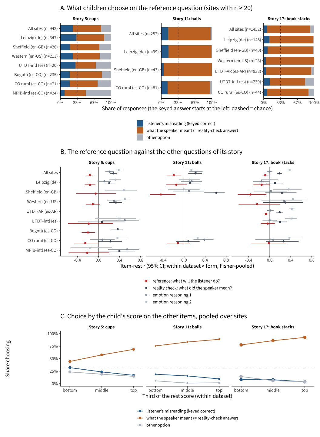
  • Keep excluded: reference_reference in stories 5, 11 and 17 (.246, .135 and .066 correct; chance .33). It is below chance in every language (cells with at least 30 responses) except German story 5, which is at chance (.317, n = 347), and its item-rest r is negative in every story. The audit found that children pick the literal referent, so a key flip would only duplicate the reality check. This is a design problem, and the items are still deployed. Story 10’s deception false belief 1 also stays excluded: its item-rest r is -.04 [-.17, .10] (n = 257), and its interval spans 0 in every language. The same generic uid covers stories 4 and 16, which discriminate and are un-excluded.
  • Scoped: story 4 on image 4g. Reality check 3 on image 4g (.188) is below chance in every language. Reality check 2 (.328) is below chance in de-DE and en-US, weak in en-GB (.300, n = 30, one-sided p = .021) and at chance in es-CO (.487), still well below its level on the earlier image 4d (.62–.66). On 4d both questions work, although reality check 3 is weak there too (.566 on two options). Both are keyed “yes” (“Is Mother/Joshua mad at Isabel now?”), but the audit found that image 4g shows Mother, Isabel and Joshua smiling, and the story never says that Mother learns what Isabel did. With the key flipped to “no”, the 4g items score .67 and .81, with item-rest r .09 [.01, .17] and .12 [.03, .20]: positive but weak (reality check 2’s interval only just clears 0), a third to a half of the 4d values (.28 and .23). The data are consistent with a key that conflicts with the scene. A scoped correction (re-key 4g to “no”) is therefore the preferred option, because it keeps the 1,243 trials, but only once the content team confirms that “no” is right for the 4g scene; exclusion is the fallback. This chapter keeps the exclusion until then.
  • Scoped: story 2 on the V0 Bogotá content. Reality check 1 on the first Bogotá content (2e, May–June 2024) is .087 (n = 229) but .915 on later content. The V0 pattern is the mirror image of the later one: 91% of V0 children chose “coats” (key “shelf”), and 91% later chose “shelf”. A flipped key would give .913, with item-rest r .11 [-.02, .24]. The mechanism is undetermined: an inverted key, a question identity swapped in the retroactive V0 map, or the V0 content itself. A clean swap of the two reality checks is not supported: the paired reality check 2 (key “coats”) drew “coats” from 66% of V0 children and 94% later. No V0 corpus survives to settle it. The scoped exclusion is the conservative choice; a key or identity correction is the alternative if the V0 content can be recovered.
  • Spanish reality_known false belief. Stories 1 and 7 still discriminate in es-CO (above), so they are un-excluded without a language flag. Story 13 does not discriminate in es-AR or es-CO and stays below the other languages at matched age; it keeps the analysis flag, but no Airtable row is proposed until the translation check. In es-AR it adds nothing to the UTDT form: reliability is .693 with it and .693 without it (2PL + guessing, empirical). The build’s spanish_fb_flag, which the analyses run with and without, still covers all three stories.
  • Un-exclude: the other 18 items behave normally; of these, story 14’s moral reality check 1 is weak.
Code
res_items$flip_check |>
  transmute(item = uid_label(story_uid), content_part, language, n, accuracy, accuracy_flipped,
            r_ir, r_ir_lo, r_ir_hi, r_ir_flipped, r_ir_flipped_lo, r_ir_flipped_hi) |>
  knitr::kable(digits = 3, caption = "Accuracy and item-rest r (within dataset × form, Fisher-pooled) with the deployed and the flipped key")
Accuracy and item-rest r (within dataset × form, Fisher-pooled) with the deployed and the flipped key
item content_part language n accuracy accuracy_flipped r_ir r_ir_lo r_ir_hi r_ir_flipped r_ir_flipped_lo r_ir_flipped_hi
S2 rc_1 flagged: 2e all 229 0.087 0.913 -0.112 -0.239 0.018 0.112 -0.018 0.239
S2 rc_1 flagged: 2e es-CO 229 0.087 0.913 -0.112 -0.239 0.018 0.112 -0.018 0.239
S2 rc_1 other content: 2f/2g and later all 719 0.915 0.085 0.210 0.134 0.284 -0.210 -0.284 -0.134
S2 rc_1 other content: 2f/2g and later de-DE 342 0.968 0.032 0.172 0.062 0.278 -0.172 -0.278 -0.062
S2 rc_1 other content: 2f/2g and later en-GB 38 0.947 0.053 0.392 0.083 0.633 -0.392 -0.633 -0.083
S2 rc_1 other content: 2f/2g and later en-US 217 0.935 0.065 0.235 0.100 0.362 -0.235 -0.362 -0.100
S2 rc_1 other content: 2f/2g and later es-CO 122 0.721 0.279 0.212 -0.001 0.407 -0.212 -0.407 0.001
S4 rc_2 flagged: 4g all 622 0.328 0.672 -0.088 -0.169 -0.005 0.088 0.005 0.169
S4 rc_2 flagged: 4g de-DE 260 0.281 0.719 -0.193 -0.309 -0.072 0.193 0.072 0.309
S4 rc_2 flagged: 4g en-GB 30 0.300 0.700 0.178 -0.195 0.506 -0.178 -0.506 0.195
S4 rc_2 flagged: 4g en-US 217 0.304 0.696 0.006 -0.133 0.144 -0.006 -0.144 0.133
S4 rc_2 flagged: 4g es-CO 115 0.487 0.513 -0.074 -0.281 0.139 0.074 -0.139 0.281
S4 rc_2 other content: 4d all 315 0.635 0.365 0.284 0.178 0.383 -0.284 -0.383 -0.178
S4 rc_2 other content: 4d de-DE 89 0.663 0.337 0.348 0.151 0.519 -0.348 -0.519 -0.151
S4 rc_2 other content: 4d es-CO 226 0.624 0.376 0.258 0.132 0.376 -0.258 -0.376 -0.132
S4 rc_3 flagged: 4g all 621 0.188 0.812 -0.117 -0.198 -0.034 0.117 0.034 0.198
S4 rc_3 flagged: 4g de-DE 260 0.158 0.842 -0.058 -0.180 0.066 0.058 -0.066 0.180
S4 rc_3 flagged: 4g en-GB 30 0.200 0.800 -0.130 -0.468 0.241 0.130 -0.241 0.468
S4 rc_3 flagged: 4g en-US 216 0.162 0.838 -0.156 -0.288 -0.017 0.156 0.017 0.288
S4 rc_3 flagged: 4g es-CO 115 0.304 0.696 -0.195 -0.390 0.016 0.195 -0.016 0.390
S4 rc_3 other content: 4d all 316 0.566 0.434 0.225 0.117 0.328 -0.225 -0.328 -0.117
S4 rc_3 other content: 4d de-DE 89 0.573 0.427 0.181 -0.028 0.375 -0.181 -0.375 0.028
S4 rc_3 other content: 4d es-CO 227 0.564 0.436 0.242 0.115 0.361 -0.242 -0.361 -0.115
Code
res_items$story2_rc_responses |>
  knitr::kable(digits = 3, caption = "Story 2's two reality checks: which option children chose, V0 Bogotá vs later content (DE trials with hostile-attribution answer strings omitted)")
Story 2’s two reality checks: which option children chose, V0 Bogotá vs later content (DE trials with hostile-attribution answer strings omitted)
entry content key response n share
reality_check_1 V0 Bogota (2e) shelf coats 209 0.913
reality_check_1 V0 Bogota (2e) shelf shelf 20 0.087
reality_check_1 later content shelf coats 54 0.086
reality_check_1 later content shelf shelf 574 0.914
reality_check_2 V0 Bogota (2e) coats coats 151 0.659
reality_check_2 V0 Bogota (2e) coats shelf 78 0.341
reality_check_2 later content coats coats 586 0.939
reality_check_2 later content coats shelf 38 0.061
ImportantWhat this means for the Airtable exclusion table

The DCC’s plan is to keep exclusions in the Airtable table, so they are documented outside code rather than written into levantemodels. The verdicts above fit that plan, with three changes:

  1. Rows need to be story-level (for example tom_story17_reference_reference), not generic. The four keep-excluded rows fit today’s columns (item_uid, exclude, dataset).
  2. Three rows need a content scope that those columns cannot express: story-4 reality checks 2 and 3 on image 4g, and story-2 reality check 1 on the V0 content (2e before 2024-07-01), that is, two content scopes covering three items. The table would need a content-version (or date-window) column. The 4g rows could instead become a key correction, which would need a place of its own (see recommendation 2).
  3. No language-scoped rows yet. Stories 1 and 7 discriminate in Spanish. Story 13 should wait for the translation check; if it then needs a Spanish row, the table would also need a language column.

The policy_exclude and spanish_fb_flag flags this chapter uses are defined in tasks/_build_stories_data.R. They stand in for those rows until the table can hold them.

Code
res_items$item_verdicts |>
  filter(!verdict %in% c("un-exclude", "un-exclude (weak item)")) |>
  transmute(item = uid_label(story_uid), verdict, proposed_airtable_row) |>
  knitr::kable(caption = glue("Proposed story-level rows other than plain un-exclusions (the other {k$v_un - k$v_es_disc} items only need their generic rows removed)"))
Proposed story-level rows other than plain un-exclusions (the other 18 items only need their generic rows removed)
item verdict proposed_airtable_row
S10 fb_1 keep excluded tom_story10_deception_false_belief_1 | all datasets
S4 rc_2 scoped exclusion tom_story4_deception_reality_check_2 | item_original 4g: exclude, or re-key to ‘no’ if the content team confirms the 4g scene
S4 rc_3 scoped exclusion tom_story4_deception_reality_check_3 | item_original 4g: exclude, or re-key to ‘no’ if the content team confirms the 4g scene
S2 rc_1 scoped exclusion tom_story2_moral_reasoning_reality_check_1 | item_original 2e before 2024-07-01 (Bogota V0): exclude
S1 fb un-exclude (below chance in Spanish, but discriminates) tom_story1_reality_known_false_belief | remove generic row
S7 fb un-exclude (below chance in Spanish, but discriminates) tom_story7_reality_known_false_belief | remove generic row
S13 fb un-exclude; flag es-* in analyses, no Airtable row until the translation check tom_story13_reality_known_false_belief | none yet (language row pending the translation check)
S5 ref keep excluded tom_story5_reference_reference | all datasets
S11 ref keep excluded tom_story11_reference_reference | all datasets
S17 ref keep excluded tom_story17_reference_reference | all datasets
Code
res_items$scoped_split |>
  transmute(item = uid_label(story_uid), scope_part, language, n, accuracy, chance,
            p_below = fp(p_below)) |>
  knitr::kable(digits = 3)
item scope_part language n accuracy chance p_below
S10 fb_1 flagged: 10d de-DE 103 0.718 0.50 1.00000
S10 fb_1 flagged: 10d en-GB 42 0.762 0.50 0.99986
S10 fb_1 flagged: 10d en-US 10 0.500 0.50 0.62305
S10 fb_1 flagged: 10d es-CO 102 0.598 0.50 0.98147
S11 ref flagged: 11b de-DE 99 0.141 0.33 < 1e-04
S11 ref flagged: 11b en-GB 43 0.047 0.33 < 1e-04
S11 ref flagged: 11b en-US 7 0.143 0.33 0.26957
S11 ref flagged: 11b es-CO 103 0.165 0.33 0.00013
S13 fb flagged: es-* es-AR 1158 0.235 0.50 < 1e-04
S13 fb flagged: es-* es-CO 97 0.289 0.50 < 1e-04
S13 fb not flagged de-DE 150 0.840 0.50 1.00000
S13 fb not flagged en-GB 36 0.472 0.50 0.43397
S13 fb not flagged en-US 10 0.400 0.50 0.37695
S17 ref flagged: 17b de-DE 148 0.115 0.33 < 1e-04
S17 ref flagged: 17b en-GB 40 0.075 0.33 0.00015
S17 ref flagged: 17b en-US 23 0.043 0.33 0.00123
S17 ref flagged: 17b es-AR 1153 0.060 0.33 < 1e-04
S17 ref flagged: 17b es-CO 88 0.068 0.33 < 1e-04
S1 fb flagged: es-* es-CO 327 0.431 0.50 0.00742
S1 fb not flagged de-DE 350 0.877 0.50 1.00000
S1 fb not flagged en-GB 26 0.885 0.50 0.99999
S1 fb not flagged en-US 221 0.620 0.50 0.99987
S2 rc_1 flagged: 2e es-CO 229 0.087 0.50 < 1e-04
S2 rc_1 not flagged de-DE 342 0.968 0.50 1.00000
S2 rc_1 not flagged en-GB 38 0.947 0.50 1.00000
S2 rc_1 not flagged en-US 217 0.935 0.50 1.00000
S2 rc_1 not flagged es-CO 122 0.721 0.50 1.00000
S4 rc_2 flagged: 4g de-DE 260 0.281 0.50 < 1e-04
S4 rc_2 flagged: 4g en-GB 30 0.300 0.50 0.02139
S4 rc_2 flagged: 4g en-US 217 0.304 0.50 < 1e-04
S4 rc_2 flagged: 4g es-CO 115 0.487 0.50 0.42608
S4 rc_2 not flagged de-DE 89 0.663 0.50 0.99933
S4 rc_2 not flagged es-CO 226 0.624 0.50 0.99993
S4 rc_3 flagged: 4g de-DE 260 0.158 0.50 < 1e-04
S4 rc_3 flagged: 4g en-GB 30 0.200 0.50 0.00072
S4 rc_3 flagged: 4g en-US 216 0.162 0.50 < 1e-04
S4 rc_3 flagged: 4g es-CO 115 0.304 0.50 < 1e-04
S4 rc_3 not flagged de-DE 89 0.573 0.50 0.93132
S4 rc_3 not flagged es-CO 227 0.564 0.50 0.97689
S5 ref flagged: 5c de-DE 89 0.180 0.33 0.00121
S5 ref flagged: 5c es-CO 226 0.195 0.33 < 1e-04
S5 ref flagged: 5c_new6 de-DE 258 0.364 0.33 0.89171
S5 ref flagged: 5c_new6 en-GB 26 0.192 0.33 0.09588
S5 ref flagged: 5c_new6 en-US 219 0.237 0.33 0.00180
S5 ref flagged: 5c_new6 es-CO 124 0.169 0.33 < 1e-04
S7 fb flagged: es-* es-CO 118 0.356 0.50 0.00112
S7 fb not flagged de-DE 102 0.922 0.50 1.00000
S7 fb not flagged en-GB 38 0.632 0.50 0.96352
S7 fb not flagged en-US 15 0.600 0.50 0.84912

The reference questions (stories 5, 11 and 17)

Each reference story asks two questions about the same request. The reality check asks what the speaker meant; the reference question asks what the listener will do, and its key is the listener’s misreading:

Code
res_mono$ref$prompts |>
  mutate(story = as.integer(str_extract(story_uid, "(?<=story)\\d+")),
         question = if_else(str_ends(story_uid, "reality_check"), "reality check", "reference")) |>
  select(story, question, prompt) |>
  pivot_wider(names_from = question, values_from = prompt) |>
  arrange(story) |>
  knitr::kable(caption = "The two questions about the request in each reference story")
The two questions about the request in each reference story
story reality check reference
5 Which cup does Katie want? Which cup will Dad give Katie?
11 Which ball does Josh want? Which ball will mom get for Josh?
17 Which stack of books was Mika talking about? Which stack of books will mom look in?
Code
rf <- res_mono$ref
ref_cl <- rf$choice_levels
ref_share <- \(s, ch, st = "All sites") pick(rf$choices, share, story == s, site == st, choice == ch)
ref_r <- \(s, col, st = "All sites") pick(rf$ir, {{ col }}, story == s, entry == "reference", site == st)
ref_icc <- \(s, th, ch = ref_cl[2]) pick(rf$icc, share, story == s, third == th, choice == ch)
ref_rc <- \(s, col) pick(rf$rc, {{ col }}, story == s)
ref_flip <- \(s) pick(rf$flip, r, story == s)
ref_age <- \(s, band, col) pick(rf$age, {{ col }}, story == s, age_band == band)
ref_sites <- rf$ir |> filter(entry == "reference", site != "All sites", n >= res_mono$meta$thresholds$MIN_N_SITE)
k$ref_cells <- nrow(ref_sites)
k$ref_cells_neg <- sum(ref_sites$r < 0)
k$ref_cells_excl <- sum(ref_sites$hi < 0)
r_ci3 <- \(s) paste0(n2(ref_r(s, r)), " [", n2(ref_r(s, lo)), ", ", n2(ref_r(s, hi)), "]")
Code
story_lab <- c(`5` = "Story 5: cups", `11` = "Story 11: balls", `17` = "Story 17: book stacks")
site_order <- c("All sites", "Leipzig (de)", "Sheffield (en-GB)", "Western (en-US)", "UTDT-AR (es-AR)",
                "UTDT-intl (es)", "Bogotá (es-CO)", "CO rural (es-CO)", "MPIB-intl (es-CO)", "LangCog (en-US)")
q_lab <- c(reference = "reference: what will the listener do?",
           reality_check = "reality check: what did the speaker mean?",
           emotion_reasoning_1 = "emotion reasoning 1", emotion_reasoning_2 = "emotion reasoning 2")
pal_choice <- set_names(c("#2c6e9b", "#c8742c", "#b9bec6"), ref_cl)
pal_q <- set_names(c("#c8342c", "#4a5462", "#8e98a4", "#c3c9d1"), q_lab)
min_site <- res_mono$meta$thresholds$MIN_N_SITE

pA <- rf$choices |>
  filter(n_site >= min_site) |>
  mutate(story = factor(story_lab[as.character(story)], story_lab),
         site_n = paste0(site, " (n=", n_site, ")"),
         site_n = fct_reorder(site_n, match(site, site_order), .desc = TRUE),
         choice = factor(choice, ref_cl)) |>
  ggplot(aes(share, site_n, fill = choice)) +
  geom_col(width = .72, position = position_stack(reverse = TRUE)) +
  geom_vline(xintercept = 1/3, linetype = "dashed", linewidth = .3) +
  facet_wrap(vars(story), scales = "free_y") +
  scale_fill_manual(values = pal_choice, name = NULL) +
  scale_x_continuous(labels = scales::percent, breaks = c(0, 1/3, 2/3, 1), expand = c(0, 0)) +
  labs(x = "Share of responses (the keyed answer starts at the left; dashed = chance)", y = NULL,
       title = glue("A. What children choose on the reference question (sites with n ≥ {min_site})")) +
  theme(legend.position = "bottom", legend.direction = "vertical")

pB <- rf$ir |>
  filter(n >= min_site, !is.na(r)) |>
  mutate(story = factor(story_lab[as.character(story)], story_lab),
         q = factor(q_lab[entry], q_lab), site = factor(site, rev(site_order))) |>
  ggplot(aes(r, site, colour = q)) +
  geom_vline(xintercept = 0, linewidth = .3) +
  geom_pointrange(aes(xmin = lo, xmax = hi), position = position_dodge(width = .7), size = .2) +
  facet_wrap(vars(story)) +
  scale_colour_manual(values = pal_q, name = NULL) +
  labs(x = "Item-rest r (95% CI; within dataset × form, Fisher-pooled)", y = NULL,
       title = "B. The reference question against the other questions of its story") +
  theme(legend.position = "bottom", legend.direction = "vertical")

pC <- rf$icc |>
  mutate(story = factor(story_lab[as.character(story)], story_lab), choice = factor(choice, ref_cl)) |>
  ggplot(aes(third, share, colour = choice)) +
  geom_hline(yintercept = 1/3, linetype = "dashed", linewidth = .3) +
  geom_line(linewidth = .8) + geom_point(aes(size = n_third)) +
  facet_wrap(vars(story)) +
  scale_colour_manual(values = pal_choice, name = NULL) +
  scale_size_area(max_size = 3, guide = "none") +
  scale_x_continuous(breaks = 1:3, labels = c("bottom", "middle", "top"), expand = expansion(add = .3)) +
  scale_y_continuous(labels = scales::percent, limits = c(0, 1)) +
  labs(x = "Third of the rest score (within dataset)", y = "Share choosing",
       title = "C. Choice by the child's score on the other items, pooled over sites") +
  theme(legend.position = "bottom", legend.direction = "vertical")

patchwork::wrap_plots(pA, pB, pC, ncol = 1, heights = c(1.1, 1.3, .8))
Figure 28.5
  • Children answer with what the speaker meant. The keyed answer is chosen by 25%, 13% and 7% of children (stories 5, 11, 17; chance 33%), and the reality-check answer by 56%, 84% and 85%.
  • Higher scorers do so more. Item-rest r is -.16 [-.23, -.10], -.20 [-.32, -.06] and -.08 [-.14, -.03]. Of the site cells with at least 20 responses, 16 of 16 have a negative point estimate, and in 6 of them the CI lies below 0. From the bottom to the top third of the rest score, the share answering with the speaker’s meaning rises from 44% to 69% (cups), 75% to 89% (balls) and 78% to 93% (book stacks). Age shows the same: on the cups story the keyed answer stays within .22–.28 in every age band from under 6 to 10 and over, while the speaker’s meaning rises from .43 to .64. The only near-chance answering comes from the youngest and lowest-scoring children.
  • Cups is the least bad, and still fails. It is at chance in Leipzig (.32), but it reverses there as well (see the screen above).
  • Flipping the key does not rescue them. Scored the other way, the questions discriminate (item-rest r .22, .23, .21), but mostly as a second copy of the reality check: children who pass it answer the reference question with the speaker’s meaning 61%, 90% and 92% of the time.
  • The rest of each story works. Its reality check and emotion questions discriminate, except story 17’s emotion reasoning 1 (see the screen above).

None of the three reference questions is worth retaining as written. One reading of the pattern is that older, higher-scoring children expect the listener to work out what the speaker meant, which may be a reasonable pragmatic inference rather than a failure to track the listener’s belief. A reference measure would need new stimuli in which the listener clearly cannot know the intended referent, piloted before deployment.

What organizes the items

Difficulty and age sensitivity

Item difficulty comes from a per-language Rasch model with guessing fixed at chance, z-scored within language. Age slopes come from item × language logistic regressions of correctness on age with dataset fixed effects. A slope needs n ≥ 50 and at least 10 correct and 10 incorrect answers.3 The R² F-tests on item × language cells treat the cells as independent, although the same item appears in several languages. The item-level rows (one value per item, averaged over languages) and the random-effects tests in the next section do not, and the text leads with them.

Code
res_items$construct_r2 |>
  filter(outcome %in% c("difficulty (IRT, z within language)", "age slope (logit per year)")) |>
  transmute(outcome, unit, scheme, n_items, R2, dR2, p = fp(p)) |>
  knitr::kable(digits = 3, caption = "Variance in item difficulty and item age slope explained by each scheme (for age slopes on cells, dR2 is over language; cell-level p-values treat cells as independent)")
Variance in item difficulty and item age slope explained by each scheme (for age slopes on cells, dR2 is over language; cell-level p-values treat cells as independent)
outcome unit scheme n_items R2 dR2 p
difficulty (IRT, z within language) item x language old_group (6) 300 0.074 0.074 0.00039
difficulty (IRT, z within language) item (mean over languages) old_group (6) 85 0.108 0.108 0.10004
age slope (logit per year) item x language (language FE; dR2 over it) old_group (6) 186 0.152 0.055 0.04764
age slope (logit per year) item (mean over languages) old_group (6) 84 0.127 0.127 0.05503
difficulty (IRT, z within language) item x language new_construct (6) 300 0.081 0.081 0.00015
difficulty (IRT, z within language) item (mean over languages) new_construct (6) 85 0.128 0.128 0.05081
age slope (logit per year) item x language (language FE; dR2 over it) new_construct (6) 186 0.183 0.086 0.00315
age slope (logit per year) item (mean over languages) new_construct (6) 84 0.169 0.169 0.01190
difficulty (IRT, z within language) item x language question_type (4) 300 0.297 0.297 < 1e-04
difficulty (IRT, z within language) item (mean over languages) question_type (4) 85 0.331 0.331 < 1e-04
age slope (logit per year) item x language (language FE; dR2 over it) question_type (4) 186 0.131 0.034 0.07453
age slope (logit per year) item (mean over languages) question_type (4) 84 0.029 0.029 0.49778
difficulty (IRT, z within language) item x language control vs target (2) 300 0.211 0.211 < 1e-04
difficulty (IRT, z within language) item (mean over languages) control vs target (2) 85 0.224 0.224 < 1e-04
age slope (logit per year) item x language (language FE; dR2 over it) control vs target (2) 186 0.098 0.001 0.70954
age slope (logit per year) item (mean over languages) control vs target (2) 84 0.004 0.004 0.55768
difficulty (IRT, z within language) item x language question_type + old_group 300 0.328 0.328 < 1e-04
difficulty (IRT, z within language) item (mean over languages) question_type + old_group 85 0.389 0.389 < 1e-04
age slope (logit per year) item x language (language FE; dR2 over it) question_type + old_group 186 0.168 0.072 0.06743
age slope (logit per year) item (mean over languages) question_type + old_group 84 0.134 0.134 0.19157
Code
sm <- res_items$scheme_means |>
  mutate(scheme = recode(scheme, question_type = "Question type", old_group = "Story type (old)",
                         new_construct = "Construct (new)"),
         scheme = factor(scheme, c("Question type", "Story type (old)", "Construct (new)")))
p_slope <- ggplot(sm, aes(x = mean_age_slope, y = fct_reorder(level, mean_age_slope))) +
  geom_linerange(aes(xmin = mean_age_slope - se_age_slope, xmax = mean_age_slope + se_age_slope)) +
  geom_point(size = 2.5) +
  facet_grid(rows = vars(scheme), scales = "free_y", space = "free_y") +
  labs(x = "Raw age slope (logit/yr, ± SE)", y = NULL) +
  theme(strip.text.y = element_blank())
p_diff <- ggplot(sm, aes(x = mean_difficulty_z, y = fct_reorder(level, mean_age_slope))) +
  geom_vline(xintercept = 0, linetype = "dotted") +
  geom_point(size = 2.5) +
  facet_grid(rows = vars(scheme), scales = "free_y", space = "free_y") +
  labs(x = "Difficulty (z within language)", y = NULL) +
  theme(axis.text.y = element_blank())
patchwork::wrap_plots(p_slope, p_diff, nrow = 1) +
  patchwork::plot_annotation(title = "Question type orders difficulty; raw age slopes (no guessing floor) barely differ")
Figure 29.1
Code
res_items$qtype_summary |>
  knitr::kable(digits = 3, caption = "By question type (item × language cells; raw logit age slopes)")
By question type (item × language cells; raw logit age slopes)
question_type n_item_lang n_items mean_accuracy mean_difficulty_z mean_age_slope median_age_slope n_slopes
false_belief 111 30 0.723 0.532 0.236 0.222 74
reality_check 99 29 0.892 -0.664 0.216 0.219 51
emotion_reasoning 75 21 0.758 -0.138 0.185 0.184 47
reference 20 5 0.676 0.804 0.113 0.132 14
Code
st <- res_items$slope_tests
spq <- res_items$slope_by_qtype |> filter(filter == "symmetric (floor model)")
k$fl_fb   <- pick(spq, mean_slope_floor, question_type == "false_belief")
k$fl_rc   <- pick(spq, mean_slope_floor, question_type == "reality_check")
k$ame_fb  <- pick(spq, mean_ame_floor, question_type == "false_belief")
k$ame_rc  <- pick(spq, mean_ame_floor, question_type == "reality_check")
k$fl_diff <- pick(st, fb_minus_control, outcome == "slope_floor", scheme == "question_type")
k$fl_lo   <- pick(st, fb_minus_control_lo, outcome == "slope_floor", scheme == "question_type")
k$fl_hi   <- pick(st, fb_minus_control_hi, outcome == "slope_floor", scheme == "question_type")
k$fl_p    <- pick(st, p, outcome == "slope_floor", scheme == "question_type")
k$raw_diff <- pick(st, fb_minus_control, outcome == "age_slope", scheme == "question_type")
k$raw_lo   <- pick(st, fb_minus_control_lo, outcome == "age_slope", scheme == "question_type")
k$raw_hi   <- pick(st, fb_minus_control_hi, outcome == "age_slope", scheme == "question_type")
k$raw_p    <- pick(st, p, outcome == "age_slope", scheme == "question_type")
k$nc_raw_p <- pick(st, p, outcome == "age_slope", scheme == "new_construct")
k$nc_fl_p  <- pick(st, p, outcome == "slope_floor", scheme == "new_construct")
ib <- \(sch, col) pick(cr, {{ col }}, outcome == "age slope (logit per year)", unit == "item (mean over languages)",
                       scheme == sch)
isl <- res_rel$item_slopes_by_type
k$a_fb <- pick(isl, median_a, question_type == "false_belief")
k$a_rc <- pick(isl, median_a, question_type == "reality_check")
asf <- res_items$age_slopes_floor
k$n_floor_fail <- sum(is.na(asf$slope_floor) & asf$cc_accuracy >= .1 & asf$cc_accuracy <= .9)
  • Difficulty is question type. Question type explains .33 of the variance across items (.30 across item × language cells); control vs target alone explains .21 across cells. Either construct scheme explains about .07. Reference and false-belief questions are hard and reality checks easy. June found the same.
  • Raw age slopes barely differ by question type. Across items, question type explains R² = .029 of the raw slopes (p = .50), and a random-effects comparison puts false belief minus controls at .003 [-.067, .073] logits per year. But raw slopes ignore the guessing floor, and their filter drops ceiling cells while keeping cells near the floor, which flattens false-belief slopes. The next section corrects both.
  • The new construct scheme’s cell-level test (ΔR² = .086, p = .003) does not hold up with item random effects (p = .05 for raw slopes, .08 above the floor).
  • Dropping the Spanish reality_known false-belief items changes none of this (see the sensitivity table below).

Age sensitivity above the guessing floor

Each item × language cell is refitted with the floor fixed at chance, P = c + (1 − c) · logistic(a + b · age), by maximum likelihood. Cells are kept symmetrically: chance-corrected accuracy between .10 and .90, n ≥ 50, SE(b) ≤ 1 (4 cells in that range did not converge). The probability-scale slope is the average marginal effect over the cell’s children. Question types are compared with a random-effects meta-regression with crossed item and language intercepts (metafor::rma.mv).

Code
res_items$slope_by_qtype |>
  select(filter, question_type, n_cells, n_items, mean_accuracy, mean_slope_logit, mean_slope_floor,
         mean_ame_logit, mean_ame_floor) |>
  knitr::kable(digits = 3, caption = "Age slopes by question type: raw logit, above the floor, and on the probability scale (per year), under the original and the symmetric filter")
Age slopes by question type: raw logit, above the floor, and on the probability scale (per year), under the original and the symmetric filter
filter question_type n_cells n_items mean_accuracy mean_slope_logit mean_slope_floor mean_ame_logit mean_ame_floor
original (>= 10 correct and incorrect) emotion_reasoning 47 21 0.726 0.185 0.217 0.029 0.026
original (>= 10 correct and incorrect) false_belief 74 30 0.666 0.236 0.435 0.038 0.033
original (>= 10 correct and incorrect) reality_check 51 28 0.834 0.216 0.301 0.024 0.022
original (>= 10 correct and incorrect) reference 14 5 0.649 0.113 1.038 0.021 0.029
symmetric (floor model) emotion_reasoning 46 21 0.721 0.190 0.223 0.029 0.027
symmetric (floor model) false_belief 52 27 0.738 0.279 0.397 0.043 0.034
symmetric (floor model) reality_check 50 29 0.841 0.211 0.276 0.023 0.021
symmetric (floor model) reference 11 5 0.682 0.167 0.316 0.032 0.029
Code
res_items$slope_tests |>
  mutate(p = fp(p)) |>
  knitr::kable(digits = 3, caption = "Random-effects tests (items and languages as crossed random intercepts; fb_minus_control from REML, 95% CI)")
Random-effects tests (items and languages as crossed random intercepts; fb_minus_control from REML, 95% CI)
outcome filter scheme n_cells n_items LR df p fb_minus_control fb_minus_control_lo fb_minus_control_hi
slope_floor symmetric question_type 159 82 13.754 3 0.0033 0.145 0.044 0.245
slope_floor symmetric new_construct 159 82 9.811 5 0.0808
slope_logit symmetric question_type 159 82 6.202 3 0.1022 0.052 -0.023 0.128
age_slope original question_type 186 84 3.540 3 0.3156 0.003 -0.067 0.073
age_slope original new_construct 186 84 11.024 5 0.0509
  • Above the floor, false-belief targets are the most age-sensitive items. Their slope is .397 logits per year against .276 for controls; the difference is .145 [.044, .245], and question type matters (p = .003). On the probability scale, false-belief accuracy rises by .034 per year against .021 for controls. The 2PL of the reliability model agrees: the median false-belief slope is 1.20, against .85 for controls.
  • So June’s “false-belief targets carry the age signal” survives, on the chance-corrected scale. On raw logits the two cannot be told apart, and controls also look flat because many are at ceiling.
Code
res_items$construct_r2_sens |>
  transmute(outcome, unit, scheme, n_items, R2, dR2, p = fp(p)) |>
  knitr::kable(digits = 3)
outcome unit scheme n_items R2 dR2 p
difficulty (IRT, z within language) item x language, es reality_known FB dropped old_group (6) 296 0.071 0.071 0.00066
age slope (logit per year) item x language, es reality_known FB dropped old_group (6) 182 0.150 0.057 0.04550
difficulty (IRT, z within language) item x language, es reality_known FB dropped new_construct (6) 296 0.078 0.078 0.00024
age slope (logit per year) item x language, es reality_known FB dropped new_construct (6) 182 0.184 0.091 0.00250
difficulty (IRT, z within language) item x language, es reality_known FB dropped question_type (4) 296 0.291 0.291 < 1e-04
age slope (logit per year) item x language, es reality_known FB dropped question_type (4) 182 0.138 0.044 0.03233
Code
res_items$construct_r2_by_lang |>
  transmute(language, outcome, scheme, n_items, R2, p = fp(p)) |>
  knitr::kable(digits = 3)
language outcome scheme n_items R2 p
de-DE difficulty old_group (6) 83 0.125 0.06186
de-DE age slope old_group (6) 47 0.237 0.04308
de-DE difficulty new_construct (6) 83 0.152 0.02417
de-DE age slope new_construct (6) 47 0.172 0.15496
de-DE difficulty question_type (4) 83 0.192 0.00073
de-DE age slope question_type (4) 47 0.076 0.33090
en-GB difficulty old_group (6) 75 0.054 0.56200
en-GB age slope old_group (6) 0 NA
en-GB difficulty new_construct (6) 75 0.054 0.56275
en-GB age slope new_construct (6) 0 NA
en-GB difficulty question_type (4) 75 0.296 < 1e-04
en-GB age slope question_type (4) 0 NA
en-US difficulty old_group (6) 28 0.213 0.34697
en-US age slope old_group (6) 28 0.141 0.61588
en-US difficulty new_construct (6) 28 0.178 0.32027
en-US age slope new_construct (6) 28 0.140 0.46061
en-US difficulty question_type (4) 28 0.483 0.00026
en-US age slope question_type (4) 28 0.023 0.74520
es-AR difficulty old_group (6) 29 0.229 0.27417
es-AR age slope old_group (6) 29 0.208 0.33609
es-AR difficulty new_construct (6) 29 0.148 0.40644
es-AR age slope new_construct (6) 29 0.205 0.22056
es-AR difficulty question_type (4) 29 0.448 0.00170
es-AR age slope question_type (4) 29 0.098 0.45250
es-CO difficulty old_group (6) 85 0.104 0.11715
es-CO age slope old_group (6) 82 0.157 0.02163
es-CO difficulty new_construct (6) 85 0.120 0.06697
es-CO age slope new_construct (6) 82 0.152 0.02581
es-CO difficulty question_type (4) 85 0.476 < 1e-04
es-CO age slope question_type (4) 82 0.101 0.03986
Code
res_items$calib_summary |>
  knitr::kable(caption = "Per-language calibrations used for item difficulty. en-US covers stories 1–6 only; en-GB rests on sparse fCAT data.")
Per-language calibrations used for item difficulty. en-US covers stories 1–6 only; en-GB rests on sparse fCAT data.
language n_runs n_items converged median_resp_per_item min_resp
de-DE 686 83 TRUE 141 89
en-GB 216 75 TRUE 38 30
en-US 257 28 TRUE 217 214
es-AR 1160 29 TRUE 1158 1139
es-CO 749 85 TRUE 104 68

Corrected question types, and story type beyond question type

The question types above come from the corpus entry names (reality_check_N, false_belief_N, …). Read against the prompts, 18 items are mislabelled. The moral questions are filed under false belief: “Is Ethan being mean and naughty?” and “Should Ethan get in trouble?” are false_belief_2 and _3 in the three moral-reasoning stories (2, 8 and 14), and the fairness question in stories 4 and 16 (“Is it fair that Mother is mad at Joshua?”) is false_belief_1. Story 10’s “Is Teacher Sarah lying?” (a false statement made in good faith; keyed “no”) is grouped with them, while “Is Brian lying?” stays a reality check. Story 16’s five questions are named reference_1–_5 although they follow story 4’s structure, so the “reference” type was not only the listener questions of stories 5, 11 and 17. Like story 4’s, they are scored by their logic: the belief-dependent “Is Dad mad at James?” as false belief, the post-reveal “… now?” as reality checks. A separate emotion-inference type was considered and not adopted: only two stories (one scenario) carry these questions, and within children the belief-dependent ones track false belief (partial r ≈ .12) more than emotion (≈ .04). Finally, the four “Does X know that …?” questions of the second-order stories (6, 12, 18) become knowledge access, a step of the Wellman and Liu theory-of-mind scale; three of them were filed as false belief. The corrected scheme (_stories_qtype_recode.R) names the moral type moral_judgment to keep it apart from the moral_reasoning story type. The table is also in the repository as stories_qtype_relabels.csv, with a note on story 10’s repeated reality check (two separate corpus rows asked at different scenes, not a serving bug).

Code
relabels |>
  transmute(status, story, story_type, entry, prompt, keyed_answer, current_type, proposed_type,
            rationale) |>
  knitr::kable(caption = "Proposed question-type relabels (rows marked proposed are applied below)")
Proposed question-type relabels (rows marked proposed are applied below)
status story story_type entry prompt keyed_answer current_type proposed_type rationale
proposed (applied in the chapter) 16 deception reference_1 Is Dad mad at James? no reference false_belief Belief-based attribution, the same structure as story 4 false_belief_2 (not a listener/reference question)
proposed (applied in the chapter) 16 deception reference_2 Is Sophie mad at James? no reference false_belief Belief-based attribution, the same structure as story 4 false_belief_3
proposed (applied in the chapter) 6 second_order false_belief_1 Does Sam know that Maria bought some socks? no false_belief knowledge_access Knowledge access (does a character know a fact?), not a false belief; easy, like the controls
proposed (applied in the chapter) 6 second_order reality_check Does Maria know that they are selling shoes in the shop? no reality_check knowledge_access Knowledge access, the counterpart question for the other character
proposed (applied in the chapter) 12 second_order false_belief_2 Does Emma know that Dad packed the blue ball? no false_belief knowledge_access Knowledge access, not a false belief
proposed (applied in the chapter) 18 second_order false_belief_2 Does George know that Kat bought a storybook? no false_belief knowledge_access Knowledge access, not a false belief
proposed (applied in the chapter) 2 moral_reasoning false_belief_2 Is Ethan being mean and naughty for taking Hannah’s book? no false_belief moral_judgment Moral judgment of the actor (blameworthiness); keyed no because the act was not intentional
proposed (applied in the chapter) 2 moral_reasoning false_belief_3 Should Ethan get in trouble with the teacher for taking Hannah’s book? no false_belief moral_judgment Moral judgment (deserved punishment); keyed no
proposed (applied in the chapter) 4 deception false_belief_1 Is it fair that Mother is mad at Joshua for losing his truck? no false_belief moral_judgment Fairness judgment about another character’s anger; keyed no
proposed (applied in the chapter) 8 moral_reasoning false_belief_2 Is Allie being mean and naughty for taking Mike’s pencil? no false_belief moral_judgment Moral judgment of the actor (blameworthiness); keyed no
proposed (applied in the chapter) 8 moral_reasoning false_belief_3 Should Allie get in trouble with the teacher for taking Mike’s pencil? no false_belief moral_judgment Moral judgment (deserved punishment); keyed no
proposed (applied in the chapter) 10 deception false_belief_1 Is Teacher Sarah lying? no false_belief moral_judgment Lie judgment: a false statement made in good faith is not a lie; keyed no
proposed (applied in the chapter) 14 moral_reasoning false_belief_2 Is Bobby being mean and naughty for taking Anna’s soccer ball? no false_belief moral_judgment Moral judgment of the actor (blameworthiness); keyed no
proposed (applied in the chapter) 14 moral_reasoning false_belief_3 Should Bobby get in trouble with their mom for taking Anna’s soccer ball? no false_belief moral_judgment Moral judgment (deserved punishment); keyed no
proposed (applied in the chapter) 16 deception false_belief_1 Is it fair that Dad is mad at Sophie for losing her shoe? no false_belief moral_judgment Fairness judgment about another character’s anger; keyed no
proposed (applied in the chapter) 16 deception reference_3 Is Dad mad at Sophie now? no reference reality_check Post-reveal check, the same structure as story 4 reality_check_1
proposed (applied in the chapter) 16 deception reference_4 Is Dad mad at James now? yes reference reality_check Post-reveal check, the same structure as story 4 reality_check_2
proposed (applied in the chapter) 16 deception reference_5 Is Sophie mad at James now? yes reference reality_check Post-reveal check, the same structure as story 4 reality_check_3
note (not relabelled) 10 deception reality_check_2 Is there still a storybook left, that isn’t being used right now? yes reality_check reality_check (keep; note) Same prompt as story 10 reality_check_3, but not served twice by mistake: separate corpus rows asked at scenes 10c and 10d, once after each lie question. 87% of children answer both the same way, so the pair is locally dependent
Code
trials |>
  filter(!policy_exclude, !is.na(age)) |>
  inner_join(res_nest$keys |> select(story_uid, question_type_v2), by = "story_uid") |>
  group_by(question_type = question_type_v2) |>
  summarise(items = n_distinct(story_uid), responses = n(), accuracy = mean(correct),
            `under 7` = mean(correct[age < 7]), `7 to 9` = mean(correct[age >= 7 & age < 9]),
            `9 and over` = mean(correct[age >= 9]), .groups = "drop") |>
  left_join(res_nest$slope_by_qtype_v2 |> select(question_type = question_type_v2,
                                                 slope_above_floor = mean_slope_floor),
            by = "question_type") |>
  knitr::kable(digits = 2, caption = "Corrected question types: accuracy by age, and the mean age slope above the guessing floor (logits per year; cells as in the floor-model section)")
Corrected question types: accuracy by age, and the mean age slope above the guessing floor (logits per year; cells as in the floor-model section)
question_type items responses accuracy under 7 7 to 9 9 and over slope_above_floor
emotion_reasoning 21 16947 0.73 0.65 0.76 0.84 0.22
false_belief 21 19076 0.60 0.47 0.64 0.76 0.43
knowledge_access 4 3410 0.88 0.80 0.92 0.94 0.43
moral_judgment 8 7413 0.72 0.63 0.73 0.85 0.31
reality_check 31 24853 0.86 0.81 0.89 0.92 0.27

Knowledge-access questions are easy, like the controls, but where they are not at ceiling they gain with age about as fast as false belief (only 7 item × language cells). Moral judgments are of medium difficulty and gain with age at .31 logits per year above the floor, between false belief (.43) and reality checks (.27).

The question that matters for story categories is not whether some story types have harder items overall, but whether stories of a given type carry additional variance once question type is controlled. The models below compare item difficulty (per-language Rasch difficulty, z within language) with and without story type, with crossed random intercepts for item and language (_stories_nested.R), and the same comparison for the age slopes above the floor as a meta-regression.

Code
res_nest$difficulty_tests |>
  transmute(question_types = qtype_scheme, comparison, df, chisq, p = fp(p), dAIC, dBIC) |>
  knitr::kable(digits = 2, caption = "Item difficulty: likelihood-ratio tests between nested models (negative dAIC/dBIC favours the larger model)")
Item difficulty: likelihood-ratio tests between nested models (negative dAIC/dBIC favours the larger model)
question_types comparison df chisq p dAIC dBIC
original story type beyond question type 5 8.53 0.1293 1.47 19.99
original individual story (random) beyond question type 1 0.00 1.0000 19.87 23.57
original question type beyond story type 3 33.07 <1e-04 -27.07 -15.96
corrected story type beyond question type 5 15.67 0.0078 -5.67 12.84
corrected individual story (random) beyond question type 1 0.00 1.0000 17.80 21.50
corrected question type beyond story type 4 44.61 <1e-04 -36.61 -21.80
Code
res_nest$item_r2 |>
  mutate(p = fp(p)) |>
  knitr::kable(digits = 3, caption = "Item level (one value per item, mean over languages): R² of each scheme, and the F test for story type beyond corrected question type")
Item level (one value per item, mean over languages): R² of each scheme, and the F test for story type beyond corrected question type
model R2 F_story_type_beyond_qt p
question type (original, 4) 0.346 NA
question type (corrected, 5) 0.335 NA
story type (6) 0.092 NA
corrected question type + story type 0.408 1.738 0.14
corrected question type + story (18) 0.490 NA
Code
res_nest$story_type_effects |>
  transmute(story_type = term, estimate, std.error) |>
  knitr::kable(digits = 2, caption = "Story-type effects on difficulty given corrected question type (relative to deception stories; z units)")
Story-type effects on difficulty given corrected question type (relative to deception stories; z units)
story_type estimate std.error
interpretation -0.75 0.28
moral_reasoning -0.27 0.24
reality_known -0.18 0.36
reference -0.54 0.32
second_order -0.59 0.30
Code
res_nest$slope_tests |>
  mutate(p = fp(p)) |>
  knitr::kable(digits = 2, caption = "Age slopes above the floor: story type beyond question type and the reverse")
Age slopes above the floor: story type beyond question type and the reverse
comparison n_cells n_items LRT df p
story type beyond question type 159 82 8.49 5 0.1313
question type beyond story type 159 82 16.69 4 0.0022
Code
nt <- res_nest$difficulty_tests |> filter(qtype_scheme == "corrected")
nt_st <- \(col) pick(nt, {{ col }}, comparison == "story type beyond question type")
nt_orig_p <- pick(res_nest$difficulty_tests, p, qtype_scheme == "original",
                  comparison == "story type beyond question type")
ir2 <- \(m) pick(res_nest$item_r2, R2, model == m)
qt_v2_label <- res_nest$item_r2$model[2]
  • For difficulty, story type adds a modest and uncertain amount beyond question type. The likelihood-ratio test gives χ²(5) = 15.7, p = .008; AIC favours adding story type (dAIC -5.7), BIC does not (dBIC 12.8). At the item level R² goes from .33 to .41 (p = .14). Given question type, items in deception stories are the hardest; items in interpretation stories are .75 SD easier and those in second-order stories .59 SD easier. Individual stories add nothing beyond item-level variation.
  • With the corpus labels the same test was not significant (p = .13), so the relabelling matters. The corrected types explain about as much difficulty variance as the corpus labels did (R² .33 vs .35); the relabelling is a correction, not a better fit.
  • For age sensitivity, story type adds nothing (p = .13), while question type does (p = .002).
  • The two schemes are only partly crossed: reference questions occur only in reference stories, moral judgments only in moral-reasoning and deception stories, and knowledge access only in second-order stories. The test is identified mainly by false-belief, reality-check and emotion items that appear across story types, with fewer than 90 items in all, so its power is limited.

Dimensionality

The factor-analytic samples are complete fixed forms, one run per child, with policy items dropped. Following June, items need coverage > .4 and .08 < p < .97. Leipzig is the June sample. Western and Bogotá give the same stories in other languages, and the UTDT no-HA retest-B form gives 1,160 es-AR children on stories 13–18.

Code
res_dim$samples |>
  transmute(sample = dim_labels[sample], role, language, stories, datasets, runs, children,
            items, age = paste0(age_min, "–", age_max, " (median ", age_median, ")"),
            n_age, first_run, last_run) |>
  knitr::kable(caption = "Dimensionality samples")
Dimensionality samples
sample role language stories datasets runs children items age n_age first_run last_run
Leipzig item bank (de-DE) primary de-DE 1-6 pilot_mpieva_de_main 275 275 23 5.1–12.9 (median 9) 275 2024-09-18 2026-02-22
Leipzig, V2 content only sensitivity de-DE 1-6 pilot_mpieva_de_main 186 186 22 5.1–12.9 (median 8.5) 186 2024-10-30 2026-02-22
Leipzig, June-style rebuild june_replication de-DE 1-6 pilot_mpieva_de_main 313 275 27 5.1–12.9 (median 9) 313 2024-09-18 2026-03-30
Western item bank (en-US) primary en-US 1-6 pilot_western_ca_main 196 196 28 5–13 (median 8.5) 196 2024-11-15 2026-04-22
Bogotá item bank (es-CO) primary es-CO 1-6 pilot_uniandes_co_bogota 229 229 25 5–12.2 (median 8.4) 151 2024-05-07 2024-06-14
Bogotá, without story-1 FB spanish_fb_variant es-CO 1-6 pilot_uniandes_co_bogota 229 229 24 5–12.2 (median 8.4) 151 2024-05-07 2024-06-14
UTDT no-HA retest-B (es-AR) primary es-AR 13-18 rfp1_utdt_ar_main, rfp1_utdt_intl_ys 1160 1160 29 4.8–8.4 (median 6.8) 1160 2026-04-29 2026-09-24
UTDT, without story-13 FB spanish_fb_variant es-AR 13-18 rfp1_utdt_ar_main, rfp1_utdt_intl_ys 1160 1160 28 4.8–8.4 (median 6.8) 1160 2026-04-29 2026-09-24
Code
res_dim$removed_items |>
  mutate(sample = dim_labels[sample], item = if_else(is.na(item), item, uid_label(item))) |>
  knitr::kable(digits = 3)
sample item reason trials runs p
Leipzig item bank (de-DE) S4 rc_2 policy_exclude 186 186 0.263
Leipzig item bank (de-DE) S4 rc_3 policy_exclude 186 186 0.140
Leipzig item bank (de-DE) S5 ref policy_exclude 275 275 0.320
Leipzig, V2 content only S4 rc_2 policy_exclude 186 186 0.263
Leipzig, V2 content only S4 rc_3 policy_exclude 186 186 0.140
Leipzig, V2 content only S5 ref policy_exclude 186 186 0.387
Leipzig, June-style rebuild no uid under this identity 255 85 0.957
Western item bank (en-US) S4 rc_2 policy_exclude 195 195 0.313
Western item bank (en-US) S4 rc_3 policy_exclude 194 194 0.160
Western item bank (en-US) S5 ref policy_exclude 195 195 0.251
Bogotá item bank (es-CO) S2 rc_1 policy_exclude 229 229 0.087
Bogotá item bank (es-CO) S5 ref policy_exclude 226 226 0.195
Bogotá, without story-1 FB S1 fb spanish_fb_flag 228 228 0.430
Bogotá, without story-1 FB S2 rc_1 policy_exclude 229 229 0.087
Bogotá, without story-1 FB S5 ref policy_exclude 226 226 0.195
UTDT no-HA retest-B (es-AR) S17 ref policy_exclude 1153 1153 0.060
UTDT, without story-13 FB S13 fb spanish_fb_flag 1158 1158 0.235
UTDT, without story-13 FB S17 ref policy_exclude 1153 1153 0.060
Code
res_dim$eigen |>
  transmute(sample = dim_labels[sample], n_items, n_persons, ev1, ev2, ev1_ev2, ev1_ev2_se,
            ev1_prop, n_ev_gt1, pa_june_nfact, pa_resample_nfact, pa_resample_ncomp, mean_offdiag_r) |>
  knitr::kable(digits = 2, caption = "Eigenvalues of the tetrachoric matrix. ev1_ev2_se is a bootstrap SE (200 person resamples). pa_june_nfact uses June's parallel analysis; pa_resample_nfact (factors) and pa_resample_ncomp (components) compare against column-resampled binary data (20 draws).")
Eigenvalues of the tetrachoric matrix. ev1_ev2_se is a bootstrap SE (200 person resamples). pa_june_nfact uses June’s parallel analysis; pa_resample_nfact (factors) and pa_resample_ncomp (components) compare against column-resampled binary data (20 draws).
sample n_items n_persons ev1 ev2 ev1_ev2 ev1_ev2_se ev1_prop n_ev_gt1 pa_june_nfact pa_resample_nfact pa_resample_ncomp mean_offdiag_r
Leipzig item bank (de-DE) 23 275 5.38 2.83 1.90 0.24 0.23 8 9 4 4 0.18
Leipzig, V2 content only 22 186 5.01 2.78 1.80 0.22 0.23 8 8 4 4 0.17
Leipzig, June-style rebuild 27 313 5.51 2.95 1.87 0.22 0.20 9 10 5 5 0.13
Western item bank (en-US) 28 196 8.14 2.73 2.99 0.36 0.29 9 12 3 2 0.25
Bogotá item bank (es-CO) 25 229 6.59 2.03 3.25 0.27 0.26 9 11 2 1 0.18
Bogotá, without story-1 FB 24 229 6.37 1.99 3.21 0.24 0.27 8 11 1 1 0.17
UTDT no-HA retest-B (es-AR) 29 1160 6.83 2.15 3.18 0.19 0.24 9 13 10 3 0.16
UTDT, without story-13 FB 28 1160 6.82 1.94 3.51 0.23 0.24 9 13 2 2 0.18
Code
res_dim$scree |>
  filter(sample %in% dim_primary, component <= 10) |>
  mutate(sample = factor(dim_labels[sample], dim_labels[dim_primary])) |>
  pivot_longer(c(eigenvalue, pa_resampled_pc), names_to = "series", values_to = "value") |>
  mutate(series = recode(series, eigenvalue = "observed",
                         pa_resampled_pc = "resampled-data reference")) |>
  ggplot(aes(component, value, linetype = series)) +
  geom_line() + geom_point(size = 1.5) +
  facet_wrap(vars(sample), nrow = 1) +
  scale_x_continuous(breaks = c(1, 5, 10)) +
  labs(x = "Component", y = "Eigenvalue", linetype = NULL,
       title = "Scree with a resampled parallel-analysis reference") +
  theme(legend.position = "bottom")
Figure 29.2
  • The Leipzig item-bank form’s ev1/ev2 (1.90, on 23 items) is close to June’s 1.90 on 26 items; the June-style rebuild gives 1.87. The Western, Bogotá and es-AR forms are at 2.99–3.25. Leipzig is near ceiling: its items average p = .82, and 11 of its 23 kept items exceed .90. Ceiling is a likely cause of the low ratio but not a tested one: the samples also differ in stories, language and age.
  • June’s parallel-analysis method gives 8–13 factors in every sample, as it gave June 11. Against resampled binary data, the primary samples need 1–4 components but 2–10 factors (es-AR: 10). Parallel analysis on tetrachoric correlations of items with a guessing floor is uninformative here: it neither supports June’s 11 nor settles on a number. The bifactor models below are the better test.

What the covariance follows: question type, story or construct

For each item pair, the tetrachoric correlation is compared within vs between groupings (June’s method). Intervals are ± 1.96 bootstrap SD over 200 person resamples. In a fixed form, story type (“old group”) gives exactly the same numbers as story, because each form has one story per story type, so it is omitted. “Question type (different stories)” compares only pairs from different stories, so it is not confounded with story.

Tetrachoric correlations are not a clean test of grouping here. Question type explains about a third of item difficulty, and items of similar difficulty with the same guessing floor correlate more on the tetrachoric scale even under one factor. The same contrasts are therefore also computed on Q3, the residual correlations after the unidimensional 2PL + guessing model of the local-dependence section, which models difficulty and guessing. Their intervals come from a person bootstrap of the residual matrix (item parameters and θ held fixed).

Code
res_dim$grouping_contrast |>
  filter(sample %in% c(dim_primary, "ar_nhb_nofb", "de_ib_junelike"), grouping != "old group") |>
  transmute(sample = dim_labels[sample], grouping, n_within, n_between, mean_within, mean_between,
            within_minus_between, diff_lo, diff_hi) |>
  knitr::kable(digits = 3, caption = "Within- minus between-group mean tetrachoric r")
Within- minus between-group mean tetrachoric r
sample grouping n_within n_between mean_within mean_between within_minus_between diff_lo diff_hi
Leipzig item bank (de-DE) story 43 210 0.202 0.174 0.027 -0.018 0.073
Leipzig item bank (de-DE) question type 98 155 0.220 0.153 0.067 0.022 0.112
Leipzig item bank (de-DE) new construct 79 174 0.181 0.178 0.003 -0.044 0.051
Leipzig item bank (de-DE) question type (different stories) 81 129 0.206 0.155 0.051 0.002 0.100
Leipzig, June-style rebuild story 59 292 0.171 0.120 0.051 0.018 0.084
Leipzig, June-style rebuild question type 114 237 0.196 0.097 0.100 0.061 0.138
Leipzig, June-style rebuild new construct 95 256 0.167 0.115 0.052 0.014 0.089
Leipzig, June-style rebuild question type (different stories) 93 199 0.174 0.096 0.078 0.036 0.120
Western item bank (en-US) story 61 317 0.250 0.244 0.005 -0.032 0.043
Western item bank (en-US) question type 127 251 0.290 0.222 0.068 0.030 0.107
Western item bank (en-US) new construct 103 275 0.224 0.253 -0.028 -0.060 0.003
Western item bank (en-US) question type (different stories) 106 211 0.278 0.227 0.051 0.009 0.092
Bogotá item bank (es-CO) story 53 247 0.189 0.172 0.017 -0.021 0.055
Bogotá item bank (es-CO) question type 117 183 0.199 0.160 0.039 0.003 0.075
Bogotá item bank (es-CO) new construct 83 217 0.161 0.180 -0.019 -0.051 0.014
Bogotá item bank (es-CO) question type (different stories) 97 150 0.182 0.165 0.017 -0.022 0.056
UTDT no-HA retest-B (es-AR) story 69 337 0.184 0.161 0.024 0.008 0.039
UTDT no-HA retest-B (es-AR) question type 95 311 0.215 0.149 0.066 0.049 0.083
UTDT no-HA retest-B (es-AR) new construct 104 302 0.187 0.157 0.030 0.014 0.045
UTDT no-HA retest-B (es-AR) question type (different stories) 73 264 0.212 0.147 0.065 0.045 0.085
UTDT, without story-13 FB story 68 310 0.191 0.177 0.014 -0.003 0.032
UTDT, without story-13 FB question type 87 291 0.230 0.165 0.065 0.048 0.083
UTDT, without story-13 FB new construct 103 275 0.192 0.175 0.016 0.000 0.033
UTDT, without story-13 FB question type (different stories) 65 245 0.231 0.163 0.068 0.047 0.089
Code
res_dim$q3_grouping_contrast |>
  filter(sample %in% dim_primary, grouping != "old group") |>
  transmute(sample = dim_labels[sample], grouping, n_within, n_between, mean_within, mean_between,
            within_minus_between, diff_lo, diff_hi) |>
  knitr::kable(digits = 3, caption = "The same contrasts on Q3 residual correlations (2PL + guessing, unidimensional)")
The same contrasts on Q3 residual correlations (2PL + guessing, unidimensional)
sample grouping n_within n_between mean_within mean_between within_minus_between diff_lo diff_hi
Leipzig item bank (de-DE) story 43 210 0.010 -0.030 0.040 0.013 0.066
Leipzig item bank (de-DE) question type 98 155 -0.019 -0.025 0.006 -0.014 0.025
Leipzig item bank (de-DE) new construct 79 174 -0.012 -0.028 0.016 -0.005 0.037
Leipzig item bank (de-DE) question type (different stories) 81 129 -0.032 -0.028 -0.004 -0.025 0.017
Western item bank (en-US) story 61 317 0.004 -0.023 0.027 0.000 0.054
Western item bank (en-US) question type 127 251 0.018 -0.037 0.056 0.029 0.082
Western item bank (en-US) new construct 103 275 -0.011 -0.022 0.010 -0.008 0.028
Western item bank (en-US) question type (different stories) 106 211 0.007 -0.038 0.045 0.019 0.071
Bogotá item bank (es-CO) story 53 247 0.019 -0.007 0.026 0.003 0.049
Bogotá item bank (es-CO) question type 117 183 0.012 -0.012 0.024 0.003 0.044
Bogotá item bank (es-CO) new construct 83 217 0.010 -0.007 0.018 -0.001 0.036
Bogotá item bank (es-CO) question type (different stories) 97 150 0.004 -0.014 0.018 -0.004 0.041
UTDT no-HA retest-B (es-AR) story 69 337 -0.003 -0.018 0.015 0.006 0.024
UTDT no-HA retest-B (es-AR) question type 95 311 0.001 -0.020 0.022 0.013 0.030
UTDT no-HA retest-B (es-AR) new construct 104 302 -0.008 -0.017 0.009 0.001 0.016
UTDT no-HA retest-B (es-AR) question type (different stories) 73 264 -0.005 -0.021 0.016 0.006 0.026
Code
res_dim$grouping_cells |>
  filter(sample %in% dim_primary) |>
  mutate(sample = factor(dim_labels[sample], dim_labels[dim_primary]),
         panel = if_else(str_detect(cell, "construct"), "Construct", "Story × type"),
         cell = fct_inorder(cell)) |>
  ggplot(aes(x = mean_r, y = fct_rev(cell), colour = sample)) +
  geom_pointrange(aes(xmin = r_lo, xmax = r_hi), position = position_dodge(width = .6)) +
  facet_grid(rows = vars(panel), scales = "free_y", space = "free_y") +
  scale_colour_manual(values = set_names(dim_pal, dim_labels[names(dim_pal)]), name = NULL) +
  labs(x = "Mean tetrachoric r (± 1.96 bootstrap SD)", y = NULL,
       title = "The 'story effect' lives in same-story, same-type pairs") +
  guides(colour = guide_legend(nrow = 2)) +
  theme(legend.position = "bottom")
Figure 29.3
Code
gc <- res_dim$grouping_contrast
qt_contrast <- gc$within_minus_between[gc$grouping == "question type" & gc$sample %in% dim_primary]
st_contrast <- gc$within_minus_between[gc$grouping == "story" & gc$sample %in% dim_primary]
nc_contrast <- gc$within_minus_between[gc$grouping == "new construct" & gc$sample %in% dim_primary]
gcell <- res_dim$grouping_cells
q3c <- res_dim$q3_grouping_contrast |> filter(sample %in% dim_primary)
q3_qt <- q3c |> filter(grouping == "question type")
q3_st <- q3c |> filter(grouping == "story")
q3_qt_ds <- q3c |> filter(grouping == "question type (different stories)")
k$q3_qt_le_story <- sum(q3_qt$within_minus_between <= q3_st$within_minus_between[match(q3_qt$sample, q3_st$sample)])
qt_ds <- gc$within_minus_between[gc$grouping == "question type (different stories)" & gc$sample %in% dim_primary]
  • Question type has a reliably positive tetrachoric contrast in every sample (.039–.068, all pairs; .017–.065 among different-story pairs), smaller than June’s .101. The June-style rebuild of the Leipzig data gives .100. That rebuild differs from the primary sample in item identities, exclusions, runs (all vs first per child) and items all at once, so the change cannot be assigned to any one of them. On Q3 residuals the question-type contrast shrinks to .006–.056 (-.004 to .045 among different-story pairs) and is no larger than the story contrast in 2 of the 4 samples. It vanishes in Leipzig (.006) and stays clearly positive in Western (.056). Part of the tetrachoric clustering by question type therefore reflects shared difficulty and guessing; what remains once they are modelled is weak and differs between samples.
  • Story contrasts are .005–.027 (Q3: .015–.040), and they come entirely from pairs of the same story and the same question type. In Leipzig, same-story pairs of the same type correlate .289; same-story pairs of different types correlate .145, no more than pairs from different stories.
  • Constructs organize little (-.028 to .030). The only test not confounded with story compares different-story pairs in the same construct with pairs across constructs. In the three stories 1–6 forms, same-construct pairs correlate less (Leipzig .157 vs .178). es-AR is the exception: its construct contrast is reliably positive (.030 [.014, .045]), and it roughly halves without the flagged story-13 item (.016). June’s table showed .045 for constructs, above story’s .039, although its prose called the construct contrast “near zero”. On Leipzig data, that contrast reproduces only on the uncorrected, June-style rebuild (.052).
  • Cleaning raised the mean inter-item correlation from .129 (June-style rebuild) to .165–.245. The defective items had depressed the between-group baseline.
Code
res_dim$efa2_summary |>
  filter(sample %in% c(dim_primary, "ar_nhb_nofb", "de_ib_junelike")) |>
  mutate(sample = dim_labels[sample]) |>
  knitr::kable(digits = 3, caption = "Two-factor oblimin EFA of the tetrachoric matrix")
Two-factor oblimin EFA of the tetrachoric matrix
sample factor_r prop_var n_items
Leipzig item bank (de-DE) 0.206 0.307 23
Leipzig, June-style rebuild 0.207 0.266 27
Western item bank (en-US) 0.391 0.348 28
Bogotá item bank (es-CO) 0.344 0.299 25
UTDT no-HA retest-B (es-AR) 0.253 0.267 29
UTDT, without story-13 FB 0.403 0.267 28
Code
res_dim$efa2_by_qtype |>
  filter(sample %in% dim_primary) |>
  mutate(sample = dim_labels[sample]) |>
  pivot_wider(names_from = sample, values_from = c(n, F1, F2), names_vary = "slowest") |>
  knitr::kable(digits = 2, caption = "Mean loadings on F1/F2 by question type")
Mean loadings on F1/F2 by question type
question_type n_UTDT no-HA retest-B (es-AR) F1_UTDT no-HA retest-B (es-AR) F2_UTDT no-HA retest-B (es-AR) n_Bogotá item bank (es-CO) F1_Bogotá item bank (es-CO) F2_Bogotá item bank (es-CO) n_Leipzig item bank (de-DE) F1_Leipzig item bank (de-DE) F2_Leipzig item bank (de-DE) n_Western item bank (en-US) F1_Western item bank (en-US) F2_Western item bank (en-US)
emotion_reasoning 7 0.34 0.09 3 0.20 0.2 5 0.19 0.25 7 0.07 0.55
false_belief 9 0.25 0.32 13 0.23 0.3 13 0.38 0.24 13 0.40 0.17
reality_check 8 0.57 -0.04 9 0.42 0.1 5 0.30 0.19 8 0.42 0.20
reference 5 0.18 0.20

A two-factor EFA still gives no sub-construct that replicates. What defines the second factor changes from sample to sample: nothing in Leipzig, an emotion factor in Western, and a split between controls and targets in es-AR.

Local dependence

A 2PL with guessing fixed at chance was fitted as a unidimensional model and as bifactor models with story testlets or question-type factors. Items answered at or below chance in the sample get a floor of 0, because a fixed floor above the observed rate cannot fit; the reliability and invariance models keep the floor at chance and are rerun under this rule as a check. Every slope has an N(0, 2²) prior (MAP-EM); without it, fixed-floor fits diverge. AIC and BIC are evaluated at the MAP estimates. dAIC and dBIC are bifactor minus unidimensional, so negative values favour the bifactor.

Code
res_dim$irt_ld |>
  filter(family == "guess", sample %in% c(dim_primary, "ar_nhb_nofb")) |>
  transmute(sample = dim_labels[sample], n_items, n_persons, dAIC_story, dBIC_story,
            dAIC_qtype, dBIC_qtype, ECV, omega_h, omega_total, omega_h_over_t = omega_h / omega_total,
            PUC, rxx_uni,
            cor_theta_uni_general, info_overstatement, q3_within_story, q3_between_story,
            `within-story pairs with Q3 > .2` = paste0(`n_within_q3_gt_.2`, "/", n_within_pairs)) |>
  knitr::kable(digits = 3, caption = "Unidimensional vs bifactor 2PL + guessing")
Unidimensional vs bifactor 2PL + guessing
sample n_items n_persons dAIC_story dBIC_story dAIC_qtype dBIC_qtype ECV omega_h omega_total omega_h_over_t PUC rxx_uni cor_theta_uni_general info_overstatement q3_within_story q3_between_story within-story pairs with Q3 > .2
Leipzig item bank (de-DE) 23 275 -41.003 42.182 -45.106 38.080 0.594 0.882 0.944 0.934 0.830 0.686 0.955 0.209 0.010 -0.030 2/43
Western item bank (en-US) 28 196 -5.148 86.639 -35.545 56.242 0.714 0.941 0.965 0.975 0.839 0.822 0.990 0.233 0.004 -0.023 6/61
Bogotá item bank (es-CO) 25 229 -3.451 78.959 -13.102 72.741 0.726 0.913 0.949 0.962 0.823 0.761 0.987 0.126 0.019 -0.007 3/53
UTDT no-HA retest-B (es-AR) 29 1160 -147.280 -0.651 -300.890 -154.261 0.639 0.894 0.959 0.932 0.830 0.776 0.989 0.149 -0.003 -0.018 2/69
UTDT, without story-13 FB 28 1160 -135.417 1.099 -156.531 -14.958 0.667 0.895 0.960 0.932 0.820 0.775 0.989 0.145 -0.001 -0.020 2/68
  • There is some story-level dependence, but little of consequence. The story bifactor improves AIC in every sample. BIC prefers the unidimensional model in the three smaller samples and is indifferent in es-AR. θ from the two models correlates .955–.990.
  • How dominant is the general factor? ECV is .59–.73, below the usual .70 guideline in Leipzig (.59) and es-AR (.64). Omega-h (.88–.94) comes from standardized normal-ogive loadings that ignore the guessing floor, so it is not comparable with the observed-score reliabilities elsewhere in this chapter. It is also inflated by story factors whose specific loadings mix signs (20 of 23 story factors in the four samples; in Leipzig story 2, Σ|λs| = 2.93 but |Σλs| = .83), and 2-item testlets are identified only through the slope prior. The ratio omega-h / omega-t (.93–.97) is the safer summary. By that ratio the general factor dominates in every sample; by ECV it dominates clearly only in Western and Bogotá, and in Leipzig and es-AR the case for it is weaker.
  • The unidimensional model overstates test information by 13%–23%, in line with the September audit’s roughly 11% on the v2_3 calibration data.
  • A question-type bifactor fits as well as the story bifactor, and in es-AR clearly better. Most of the es-AR advantage comes from the below-chance Spanish false-belief item: without story 13’s item, dBIC for the question-type model goes from -154 to -15.

The residual dependence sits in a handful of “doublets”. Most are yes/no questions about the same scene with the same key. One pair of location false-belief questions from different stories behaves the same way:

Code
res_dim$ld_pairs_top |>
  filter(sample %in% dim_primary) |>
  transmute(sample = dim_labels[sample], item_i = uid_label(i), item_j = uid_label(j),
            same_story, r, q3, code_i, answer_i, p_i, code_j, answer_j, p_j) |>
  knitr::kable(digits = 2, caption = "Item pairs with Q3 > .2 (2PL + guessing, unidimensional)")
Item pairs with Q3 > .2 (2PL + guessing, unidimensional)
sample item_i item_j same_story r q3 code_i answer_i p_i code_j answer_j p_j
UTDT no-HA retest-B (es-AR) S13 fb S14 fb_1 FALSE 0.52 0.34 13c box 0.23 14d table 0.37
UTDT no-HA retest-B (es-AR) S16 ref_4 S16 ref_5 TRUE 0.54 0.30 16f yes 0.68 16f yes 0.59
UTDT no-HA retest-B (es-AR) S14 fb_2 S14 fb_3 TRUE 0.38 0.21 14g no 0.60 14g no 0.55
Bogotá item bank (es-CO) S4 rc_2 S4 rc_3 TRUE 0.68 0.44 4d yes 0.62 4d yes 0.56
Bogotá item bank (es-CO) S6 fb_2 S6 fb_5 TRUE 0.81 0.43 6c shoes 0.46 6d shoes 0.44
Bogotá item bank (es-CO) S1 fb S2 fb_1 FALSE 0.68 0.36 1c chair 0.43 2d shelf 0.53
Bogotá item bank (es-CO) S4 fb_2 S4 fb_3 TRUE 0.42 0.26 4c no 0.61 4c no 0.46
Bogotá item bank (es-CO) S3 fb S6 fb_4 FALSE 0.41 0.21 3d tree 0.60 6d shirts 0.41
Bogotá item bank (es-CO) S5 rc S6 fb_4 FALSE 0.41 0.21 5c large_cup 0.61 6d shirts 0.41
Bogotá item bank (es-CO) S1 rc S3 rc_2 FALSE 0.69 0.20 1c rug 0.86 3d fountain 0.94
Leipzig item bank (de-DE) S6 fb_2 S6 fb_5 TRUE 0.76 0.44 6c_new2 shoes 0.73 6d_new2 shoes 0.67
Leipzig item bank (de-DE) S4 fb_2 S4 fb_3 TRUE 0.69 0.43 4c_new3 no 0.61 4c_new3 no 0.51
Leipzig item bank (de-DE) S1 fb S2 fb_1 FALSE 0.79 0.31 1c chair 0.86 2d shelf 0.92
Leipzig item bank (de-DE) S4 er_2 S5 er_2 FALSE 0.68 0.31 4b_new2 happy 0.87 5d happy 0.95
Leipzig item bank (de-DE) S5 rc S6 fb_1 FALSE 0.62 0.27 5c_new6 large_cup 0.93 6c_new2 no 0.96
Western item bank (en-US) S2 fb_2 S2 fb_3 TRUE 0.71 0.45 2f_new2 no 0.77 2f_new2 no 0.77
Western item bank (en-US) S2 rc_1 S2 rc_2 TRUE 0.65 0.34 2g shelf 0.94 2f_new2 coats 0.94
Western item bank (en-US) S6 fb_2 S6 fb_5 TRUE 0.67 0.30 6c_new2 shoes 0.61 6d_new2 shoes 0.56
Western item bank (en-US) S1 rc S3 rc_2 FALSE 0.52 0.25 1c rug 0.92 3d behind-fountain 0.94
Western item bank (en-US) S4 er_1 S5 er_1 FALSE 0.65 0.23 4b_new2 sad 0.89 5d sad 0.93
Western item bank (en-US) S5 er_1 S5 er_2 TRUE 0.73 0.22 5d sad 0.93 5d happy 0.85
Western item bank (en-US) S4 fb_2 S4 fb_3 TRUE 0.33 0.22 4c_new3 no 0.74 4c_new3 no 0.45
Western item bank (en-US) S4 er_1 S4 er_2 TRUE 0.69 0.21 4b_new2 sad 0.89 4b_new2 happy 0.77
Code
res_dim$irt_ld |>
  filter(family == "noguess") |>
  transmute(sample = dim_labels[sample], dAIC_story, dBIC_story, dAIC_qtype, dBIC_qtype,
            ECV, omega_h, cor_theta_uni_general, info_overstatement) |>
  knitr::kable(digits = 3)
sample dAIC_story dBIC_story dAIC_qtype dBIC_qtype ECV omega_h cor_theta_uni_general info_overstatement
Leipzig item bank (de-DE) -131.687 -48.501 -46.850 36.336 0.497 0.829 0.961 0.110
Leipzig, V2 content only -87.967 -17.000 -51.252 19.715 0.492 0.817 0.954 0.178
Leipzig, June-style rebuild -167.990 -66.842 -156.662 -59.261 0.466 0.794 0.973 0.055
Western item bank (en-US) -76.569 15.218 -77.447 14.340 0.625 0.912 0.992 0.078
Bogotá item bank (es-CO) -71.619 10.790 -73.753 12.091 0.615 0.844 0.978 0.107
Bogotá, without story-1 FB -69.591 5.951 -57.151 25.259 0.619 0.841 0.979 0.100
UTDT no-HA retest-B (es-AR) -261.083 -114.453 -416.052 -269.423 0.640 0.865 0.995 0.055
UTDT, without story-13 FB -245.392 -108.876 -298.937 -157.364 0.681 0.867 0.996 0.054

Sub-scales

Code
res_dim$subscales |>
  filter(sample %in% dim_primary) |>
  transmute(sample = dim_labels[sample], scale, n_items, alpha, alpha_sb_to_all,
            twopl_marginal_rxx, rasch_marginal_rxx, age_r, age_r_lo, age_r_hi,
            pct_rand_alpha_below, pct_rand_age_r_below) |>
  knitr::kable(digits = 3, caption = "Sub-scales. alpha_sb_to_all projects alpha to the full scale's length (Spearman–Brown). pct_rand_* is the percentile among 500 random item subsets of the same size.")
Sub-scales. alpha_sb_to_all projects alpha to the full scale’s length (Spearman–Brown). pct_rand_* is the percentile among 500 random item subsets of the same size.
sample scale n_items alpha alpha_sb_to_all twopl_marginal_rxx rasch_marginal_rxx age_r age_r_lo age_r_hi pct_rand_alpha_below pct_rand_age_r_below
Leipzig item bank (de-DE) all items 23 0.675 0.675 0.643 0.719 0.429 0.328 0.521
Leipzig item bank (de-DE) targets only 18 0.664 0.716 0.642 0.695 0.438 0.338 0.529 0.980 0.736
Leipzig item bank (de-DE) false-belief only 13 0.637 0.756 0.606 0.584 0.434 0.333 0.525 0.994 0.766
Leipzig item bank (de-DE) controls only 5 0.180 0.502 0.140 0.211 0.107 -0.011 0.222 0.146 0.034
Western item bank (en-US) all items 28 0.805 0.805 0.769 0.738 0.550 0.444 0.640
Western item bank (en-US) targets only 20 0.764 0.819 0.744 0.729 0.554 0.449 0.644 0.812 0.902
Western item bank (en-US) false-belief only 13 0.727 0.851 0.706 0.616 0.535 0.427 0.628 0.990 0.854
Western item bank (en-US) controls only 8 0.558 0.815 0.383 0.176 0.324 0.193 0.444 0.610 0.014
Bogotá item bank (es-CO) all items 25 0.734 0.734 0.794 0.871 0.428 0.288 0.550
Bogotá item bank (es-CO) targets only 16 0.657 0.750 0.727 0.815 0.429 0.289 0.551 0.668 0.734
Bogotá item bank (es-CO) false-belief only 13 0.649 0.780 0.711 0.769 0.451 0.314 0.570 0.832 0.906
Bogotá item bank (es-CO) controls only 9 0.518 0.749 0.570 0.658 0.299 0.146 0.437 0.604 0.236
UTDT no-HA retest-B (es-AR) all items 29 0.703 0.703 0.736 0.883 0.455 0.408 0.500
UTDT no-HA retest-B (es-AR) targets only 21 0.641 0.712 0.703 0.883 0.432 0.384 0.477 0.682 0.526
UTDT no-HA retest-B (es-AR) false-belief only 9 0.550 0.797 0.608 0.657 0.354 0.303 0.404 0.946 0.480
UTDT no-HA retest-B (es-AR) controls only 8 0.523 0.799 0.409 0.229 0.313 0.260 0.364 0.926 0.258
Code
ss <- res_dim$subscales |> filter(sample %in% dim_primary) |>
  mutate(sample = factor(dim_labels[sample], dim_labels[dim_primary]),
         scale = factor(scale, c("all items", "targets only", "false-belief only", "controls only")))
ggplot(ss, aes(x = scale, y = age_r)) +
  geom_linerange(aes(ymin = rand_age_r_q025, ymax = rand_age_r_q975), linewidth = 4,
                 colour = "grey80", data = filter(ss, scale != "all items")) +
  geom_pointrange(aes(ymin = age_r_lo, ymax = age_r_hi)) +
  facet_wrap(vars(sample), nrow = 1) +
  scale_x_discrete(limits = levels(ss$scale)) +
  labs(x = NULL, y = "r(proportion correct, age)",
       title = "Age validity of sub-scales against random item subsets of the same size (grey)") +
  theme(axis.text.x = element_text(angle = 30, hjust = 1))
Figure 29.4

June’s answer stands: no sub-scale improves on the full set. False-belief items are the most internally consistent per item (Spearman–Brown-projected alpha .76–.85), but a false-belief-only scale is no more age-valid than random subsets. In es-AR it is less age-valid than the full scale. The controls are the least age-valid items (discussed next).

Controls

This section re-tests June’s claims about the reality-check (control) questions: that they correlate with targets, that they do not gate the targets’ age sensitivity, and that keeping them helps reliability.

Code
res_items$controls_cor |>
  knitr::kable(digits = 3, caption = "Person-level correlations of control and target accuracy (runs with age)")
Person-level correlations of control and target accuracy (runs with age)
method item_set n_runs r_control_target r_control_age r_target_age n_cells r_control_target_lo r_control_target_hi r_control_target_partial_age
pooled over runs (June method) policy items dropped 3016 0.483 0.222 0.492
pooled over runs (June method) all items (June item set) 3016 0.384 0.147 0.486
within dataset x form, Fisher-pooled policy items dropped 2972 0.344 0.130 0.288 16 0.312 0.376 0.324
within dataset x form, Fisher-pooled all items (June item set) 2972 0.296 0.145 0.285 16 0.263 0.329 0.265
Code
res_items$controls_cells |>
  mutate(dataset = ds_label(dataset)) |>
  select(-cell) |>
  knitr::kable(digits = 3)
dataset form language n_runs median_items median_ctrl mean_control mean_target r_control_target r_control_age r_target_age r_control_target_partial_age
Germany — Leipzig fcat_random3 de-DE 182 13 4 0.969 0.877 0.019 -0.032 0.167 0.025
Germany — Leipzig item_bank de-DE 313 28 8 0.946 0.803 0.258 0.034 0.398 0.267
Germany — Leipzig retest_A de-DE 69 26 11 0.967 0.913 0.389 0.147 0.272 0.366
Germany — Leipzig retest_B de-DE 112 29 8 0.962 0.839 0.265 -0.160 0.361 0.351
Colombia — Bogotá fcat_random3 es-CO 39 13 4 0.878 0.670 0.591 0.354 0.543 0.508
Colombia — Bogotá item_bank es-CO 151 25 9 0.700 0.610 0.541 0.299 0.429 0.479
Colombia — Caquetá/Boyacá co_retest_A es-CO 44 29 11 0.871 0.766 0.316 0.142 -0.285 0.376
Colombia — Caquetá/Boyacá fcat_random3 es-CO 216 14 4 0.860 0.661 0.395 0.300 0.439 0.307
Colombia — Caquetá/Boyacá item_bank es-CO 32 28 8 0.680 0.407 0.018 -0.076 0.011 0.019
Canada — Ontario fcat_random3 en-US 76 14 4 0.921 0.710 0.398 0.330 0.583 0.268
Canada — Ontario item_bank en-US 201 28 8 0.912 0.718 0.559 0.325 0.554 0.482
Germany — MPIB (RfP1 YS) fcat_random3 es-CO 75 14 4 0.706 0.463 0.295 0.244 -0.052 0.318
UK — Sheffield fcat_random3 en-GB 216 14 4 0.944 0.782 0.274 0.003 0.225 0.281
Argentina — UTDT (main) no_ha_retest_B es-AR 943 29 8 0.926 0.668 0.354 0.096 0.221 0.343
Argentina — UTDT (RfP1 YS) fcat_random3 es-CO 86 13 4 0.698 0.458 0.375 0.145 0.254 0.354
Argentina — UTDT (RfP1 YS) no_ha_retest_B es-AR 217 29 8 0.808 0.501 0.324 0.200 0.077 0.315

Pooled over runs, as June did it, control and target accuracy correlate .48. Much of that is between-site differences: within dataset × form the correlation is .34, and controls correlate .13 with age. These are accuracy scores, and fCAT runs have a median of 4 controls each, which attenuates the correlations.

Gating

Code
res_items$gating_june |> select(-method) |>
  knitr::kable(digits = 3, caption = "June method: lm(story target accuracy ~ scale(age)) by whether the story's control was passed")
June method: lm(story target accuracy ~ scale(age)) by whether the story’s control was passed
ctrl_pass n_story_instances mean_target_acc mean_age target_age_beta_perSD
FALSE 1980 0.539 7.195 0.088
TRUE 11691 0.691 7.991 0.106
Code
res_items$gating_glmm |>
  mutate(interaction_p = fp(interaction_p)) |>
  knitr::kable(digits = 3, caption = "GLMM on target trials: correct ~ age × ctrl_pass + dataset + (1 | run) + (1 | story_uid). Slopes in logits per year.")
GLMM on target trials: correct ~ age × ctrl_pass + dataset + (1 | run) + (1 | story_uid). Slopes in logits per year.
sample n_trials n_runs pct_instances_fail pass_effect_at_age8 age_slope_fail age_slope_fail_se age_slope_pass age_slope_pass_se interaction interaction_se interaction_p singular
all languages 38812 3016 14.483 0.449 0.172 0.019 0.215 0.011 0.043 0.019 0.020 FALSE
de-DE 9895 686 6.084 0.300 -0.027 0.049 0.199 0.019 0.226 0.050 <1e-04 FALSE
en-GB 1709 216 8.007 1.393 -0.115 0.189 0.285 0.072 0.401 0.199 0.044 FALSE
en-US 4742 284 11.462 0.454 0.174 0.054 0.313 0.027 0.138 0.054 0.010 FALSE
es-AR 14993 1160 14.110 0.623 0.199 0.068 0.317 0.044 0.118 0.061 0.052 FALSE
es-CO 7473 670 29.616 0.275 0.215 0.028 0.179 0.020 -0.035 0.028 0.210 FALSE
Code
res_items$gating_plot |>
  mutate(language = factor(language, lang_levels),
         ctrl_pass = if_else(ctrl_pass, "control passed", "control failed")) |>
  ggplot(aes(age_bin, target_acc, colour = ctrl_pass)) +
  geom_line() + geom_point(aes(size = n), alpha = .7) +
  facet_wrap(vars(language), nrow = 1) +
  scale_size_area(max_size = 4, guide = "none") +
  scale_colour_manual(values = c("control passed" = "grey30", "control failed" = "#CC6677"),
                      name = NULL) +
  labs(x = "Age (years)", y = "Target accuracy in the story",
       title = "Target accuracy by age, split by whether the story's control was passed") +
  theme(legend.position = "bottom")
Figure 30.1
Code
gg <- res_items$gating_glmm
g_all <- filter(gg, sample == "all languages"); g_de <- filter(gg, sample == "de-DE")
g_co  <- filter(gg, sample == "es-CO")
gj <- res_items$gating_june

June’s method again finds no gating: the target age slope is .088 per SD of age after a failed control and .106 after a passed one. The trial-level GLMM finds a small pooled interaction (.043 logits/yr, p = .020). It comes from de-DE, where targets after a failed control show no age slope (-.027 vs .199; 6.1% of story instances failed), and to a lesser degree from en-US (.138, p = .010); en-GB and es-AR are borderline (p = .044 and .052). es-CO shows none (29.6% failed). Passing a control is itself related to ability, so this is a description, not a causal gate. In a high-scoring sample like Leipzig, a failed control probably marks a lapse.

Do controls help the score?

On fixed forms, with guessing fixed at chance and production priors:

Code
res_items$reliability |>
  mutate(row = row_number()) |>
  filter(row %in% c(1:8, 13:14)) |>
  select(sample, items, model, guessing, n_runs, n_items, n_controls, mean_items_answered,
         marginal_rxx_mirt, marginal_rxx, empirical_rxx, alpha_complete_cases,
         r_theta_age, r_theta_all_vs_targets) |>
  knitr::kable(digits = 3, caption = "Reliability and age validity with and without controls. The last two rows replicate June's method: pure Rasch without priors on June's 58-item Leipzig pool (item bank and retest forms, released identities, policy items kept).")
Reliability and age validity with and without controls. The last two rows replicate June’s method: pure Rasch without priors on June’s 58-item Leipzig pool (item bank and retest forms, released identities, policy items kept).
sample items model guessing n_runs n_items n_controls mean_items_answered marginal_rxx_mirt marginal_rxx empirical_rxx alpha_complete_cases r_theta_age r_theta_all_vs_targets
DE Leipzig, item-bank form (stories 1-6) all items Rasch fixed at chance 313 30 10 27.383 0.455 0.680 0.651 0.640 0.377 0.964
DE Leipzig, item-bank form (stories 1-6) targets only Rasch fixed at chance 313 20 0 18.818 0.384 0.647 0.625 0.611 0.394 0.964
DE Leipzig, item-bank form (stories 1-6) all items 2PL fixed at chance 313 30 10 27.383 0.622 0.622 0.638 0.640 0.394 0.968
DE Leipzig, item-bank form (stories 1-6) targets only 2PL fixed at chance 313 20 0 18.818 0.579 0.579 0.602 0.611 0.411 0.968
UTDT-AR main, no-HA retest-B form (stories 13-18) all items Rasch fixed at chance 943 29 8 28.925 0.560 0.674 0.669 0.656 0.190 0.945
UTDT-AR main, no-HA retest-B form (stories 13-18) targets only Rasch fixed at chance 943 21 0 20.947 0.521 0.596 0.591 0.605 0.197 0.945
UTDT-AR main, no-HA retest-B form (stories 13-18) all items 2PL fixed at chance 943 29 8 28.925 0.667 0.667 0.693 0.656 0.200 0.950
UTDT-AR main, no-HA retest-B form (stories 13-18) targets only 2PL fixed at chance 943 21 0 20.947 0.603 0.603 0.628 0.605 0.213 0.950
DE Leipzig, June item pool (June method) all items Rasch none 425 58 16 27.894 0.922 0.712 0.554 0.389 0.942
DE Leipzig, June item pool (June method) targets only Rasch none 425 42 0 19.400 0.893 0.709 0.542 0.366 0.942
Code
rrow <- \(s, it, m, col) pick(res_items$reliability, {{ col }}, sample == s, items == it, model == m)
de_s <- "DE Leipzig, item-bank form (stories 1-6)"
ar_s <- "UTDT-AR main, no-HA retest-B form (stories 13-18)"
jn_s <- "DE Leipzig, June item pool (June method)"
# the items script and the dimensionality script replicate June's .92 on the same pool
stopifnot(abs(rrow(jn_s, "all items", "Rasch", marginal_rxx_mirt) - jp$rasch_marginal_rxx_june_method) < .001,
          abs(rrow(jn_s, "all items", "Rasch", empirical_rxx) - jp$rasch_empirical_rxx_eap) < .001)
k$dage_max <- res_items$reliability |> slice(1:8) |>
  select(sample, model, items, r_theta_age) |>
  pivot_wider(names_from = items, values_from = r_theta_age) |>
  summarise(d = max(abs(`all items` - `targets only`))) |> pull(d)
  • Keep the controls. They raise reliability a little: Leipzig .651 with them vs .625 without; UTDT .669 vs .591 (Rasch + guessing, empirical). They change r(θ, age) by at most .02. June reached the same conclusion.
  • Per item, controls are the weakest. The dimensionality analysis finds them the least age-valid items. In Leipzig a controls-only score correlates .107 with age, below 97% of random 5-item subsets. Once alpha is projected to equal length, targets alone match all items in every sample. Controls help the score as extra items, not as especially good ones.
  • June’s .92 → .89. That comparison reproduces as mirt’s marginal_rxx on June’s sparse 58-item Leipzig pool (.922 with controls vs .893 without; June: .915 vs .885). Children answered 27.9 of those items on average. The same fit’s empirical reliability is .554 with controls and .542 without. mirt::marginal_rxx() integrates TI/(TI + var) over N(0, 1) and assumes every item is answered. With a Rasch latent variance of .44, that inflates the value. The reliability section returns to this.

Cross-language invariance

Methods. Multigroup Rasch with the guessing floor fixed at chance (the LEVANTE convention), fitted with mirt. Each child contributes one run: the earliest that contains the analysed stories. An item needs ≥ 100 responses per group. The sequence is configural vs scalar, then a DIF screen with all other items as anchors, then purified and iterated anchors, then partial scalar. fCAT runs are included; their missing items are missing by design. Effect sizes db are item difficulty for a group minus de-DE, in logits; positive means harder at matched ability. dBIC = BIC(constrained) − BIC(less constrained), so positive values favour the less constrained model.

The ETS classes are adapted, not the ETS rule itself: A (negligible), B (moderate) and C (large) use the 1- and 1.5-delta cut-offs (0.43 and 0.64 logits) on latent-logit db under the guessing floor, which runs larger than the observed-score Mantel–Haenszel D-DIF they were defined for. Significance is the item’s BH-adjusted LR test, and class C does not require |db| to be significantly above 0.43.

A maximum-likelihood 2PL was not usable: its configural models do not converge, and slopes reach 41. A 2PL with the production priors (d ~ N(0, 3), a ~ N(1, 0.3), MAP) is usable and serves as the second model throughout: for the metric and scalar tests, and for DIF effect sizes.

Code
res_inv$model_choice |>
  select(analysis, model, logLik, npar, BIC, converged, iterations, max_slope,
         prop_slopes_over_4, prop_slopes_negative) |>
  knitr::kable(digits = 2, caption = "Maximum-likelihood 2PL + guessing fits are degenerate")
Maximum-likelihood 2PL + guessing fits are degenerate
analysis model logLik npar BIC converged iterations max_slope prop_slopes_over_4 prop_slopes_negative
A Rasch+g configural -9946.18 84 20485.44 TRUE 32 1.00 0.00 0.00
A Rasch+g scalar -10133.36 32 20492.66 TRUE 36 1.00 0.00 0.00
A 2PL+g configural -9792.60 162 20728.99 FALSE 5000 21.16 0.22 0.04
A 2PL+g metric -9842.83 110 20462.31 TRUE 233 40.94 0.11 0.00
A 2PL+g scalar -9993.30 58 20396.11 TRUE 85 22.63 0.15 0.00
B Rasch+g configural -17295.93 56 34995.62 TRUE 39 1.00 0.00 0.00
B Rasch+g scalar -17473.54 30 35163.37 TRUE 83 1.00 0.00 0.00
B 2PL+g configural -17021.70 108 34822.09 FALSE 5000 9.47 0.15 0.07
B 2PL+g metric -17045.20 82 34681.63 TRUE 313 14.30 0.11 0.04
B 2PL+g scalar -17152.82 56 34709.41 TRUE 368 40.72 0.11 0.04
Code
res_inv$samples |>
  filter(analysis %in% c("A", "B")) |>
  select(analysis, group, n_children, age_median, age_q1, age_q3, age_missing, datasets, forms) |>
  knitr::kable(digits = 1, caption = "Analysis A: stories 1–6, de-DE vs en-US vs es-CO. Analysis B: stories 13–18, de-DE vs es-AR.")
Analysis A: stories 1–6, de-DE vs en-US vs es-CO. Analysis B: stories 13–18, de-DE vs es-AR.
analysis group n_children age_median age_q1 age_q3 age_missing datasets forms
A de_DE 301 9.0 7.1 10.9 0 pilot_mpieva_de_main, rfp1_mpib_de_main item_bank, fcat_random3, no_ha
A en_US 247 7.8 6.4 10.1 0 pilot_langcog_us_downex, pilot_western_ca_main item_bank, fcat_random3
A es_CO 617 7.9 6.0 10.2 79 pilot_uniandes_co_bogota, pilot_uniandes_co_rural, rfp1_mpib_intl_ys, rfp1_utdt_intl_ys fcat_random3, item_bank, co_retest_A, co_retest_B
B de_DE 193 9.9 7.3 11.7 0 pilot_mpieva_de_main, rfp1_mpib_de_main retest_B, fcat_random3
B es_AR 1160 6.8 6.2 7.5 0 rfp1_utdt_ar_main, rfp1_utdt_intl_ys no_ha_retest_B
Code
sB <- res_inv$samples |> filter(analysis == "B")
# how many earlier included ToM runs each analysed child had (the analysed run is the child's
# earliest run containing the analysed stories)
inc_runs <- runs |> filter(included) |> arrange(user_id, time_started) |>
  group_by(user_id) |> mutate(k_run = row_number()) |> ungroup()
first_with <- \(st, langs) trials |>
  filter(story %in% st, language %in% langs, !policy_exclude) |>
  distinct(user_id, run_id, time_started, language) |>
  arrange(time_started, run_id) |> group_by(user_id) |> slice(1) |> ungroup() |>
  left_join(inc_runs |> select(run_id, k_run), by = "run_id")
expB <- first_with(13:18, c("de-DE", "es-AR")) |>
  left_join(runs |> select(run_id, age), by = "run_id")
k$B_de_n <- sum(expB$language == "de-DE")
k$B_de_repeat <- sum(expB$language == "de-DE" & expB$k_run > 1)
k$B_ar_repeat <- sum(expB$language == "es-AR" & expB$k_run > 1)
k$Byoung_n <- sum(expB$language == "de-DE" & !is.na(expB$age) & expB$age < 9)
k$Byoung_repeat <- sum(expB$language == "de-DE" & !is.na(expB$age) & expB$age < 9 & expB$k_run > 1)
stopifnot(k$B_de_n == pick(sB, n_children, group == "de_DE"),
          k$Byoung_n == pick(res_inv$samples, n_children, analysis == "B_young", group == "de_DE"))

The groups are not language groups only. In stories 13–18 (analysis B), 168 of the 193 German children (87%) were on their second or third ToM run, having taken stories 1–6 or 7–12 earlier; none of the es-AR children were. The German children are older (median 9.9 vs 6.8 years), and es-AR comes from one site (UTDT). In A, the German children are older too, and es-CO pools four datasets from 2024–2026, including the V0 content. Group differences in item difficulty are therefore differences between samples that differ in language, age, prior exposure and site, and the estimated group means (numerics note) are not language differences in theory of mind.

Code
res_inv$tests |>
  filter(analysis %in% c("A", "B")) |>
  transmute(analysis, comparison, items, n_items, X2, df, X2_df, p = fp(p), dBIC) |>
  knitr::kable(digits = 2, caption = "Invariance tests, Rasch + guessing")
Invariance tests, Rasch + guessing
analysis comparison items n_items X2 df X2_df p dBIC
A scalar vs configural all 27 374.37 52 7.20 <1e-04 7.22
A partial scalar vs configural all 27 35.32 28 1.26 0.1606 -162.37
A scalar vs partial scalar all 27 339.04 24 14.13 <1e-04 169.59
A scalar vs configural targets 20 237.03 38 6.24 <1e-04 -31.27
A partial scalar vs configural targets 20 25.01 20 1.25 0.2009 -116.20
A scalar vs configural controls 7 84.01 12 7.00 <1e-04 -0.46
A partial scalar vs configural controls 7 17.45 6 2.91 0.0078 -24.79
B scalar vs configural all 27 355.21 26 13.66 <1e-04 167.75
B partial scalar vs configural all 27 20.66 19 1.09 0.3559 -116.33
B scalar vs partial scalar all 27 334.55 7 47.79 <1e-04 284.08
B scalar vs configural targets 20 338.79 19 17.83 <1e-04 201.80
B partial scalar vs configural targets 20 18.28 13 1.41 0.1471 -75.45
B scalar vs configural controls 7 11.40 6 1.90 0.0767 -31.84
B partial scalar vs configural controls 7 6.33 5 1.27 0.2752 -29.71
Code
res_inv$tests_2pl |>
  transmute(analysis, comparison, df, X2_logLik, X2_logpost, p_logpost = fp(p_logpost), dBIC,
            nested_optimum_better) |>
  knitr::kable(digits = 2, caption = "Invariance tests, 2PL + guessing with production priors (MAP). X2 on the log-likelihood and on the log posterior; dBIC from mirt's BIC. A more constrained model reaching a better optimum (nested_optimum_better) means the less constrained fit found a local optimum, so only metric vs scalar is interpreted.")
Invariance tests, 2PL + guessing with production priors (MAP). X2 on the log-likelihood and on the log posterior; dBIC from mirt’s BIC. A more constrained model reaching a better optimum (nested_optimum_better) means the less constrained fit found a local optimum, so only metric vs scalar is interpreted.
analysis comparison df X2_logLik X2_logpost p_logpost dBIC nested_optimum_better
A metric vs configural 52 -93.25 -92.87 1.00 -460.39 TRUE
A scalar vs metric 52 299.15 55.58 0.34 -67.99 FALSE
B metric vs configural 26 -57.58 -82.88 1.00 -245.04 TRUE
B scalar vs metric 26 274.56 165.58 <1e-04 87.09 FALSE
Code
t2 <- \(a, cmp, col) pick(res_inv$tests_2pl, {{ col }}, analysis == a, comparison == cmp)
tr_ <- \(a, cmp, col, it = "all") pick(tst, {{ col }}, analysis == a, comparison == cmp, items == it)
isl <- res_rel$item_slopes_by_type
dlab <- res_inv$dif_long |> filter(analysis %in% c("A", "B"))
k$mdd_med <- median(dlab$mdd, na.rm = TRUE)
k$se_med  <- median(dlab$se, na.rm = TRUE)
k$mdd_B   <- median(dlab$mdd[dlab$analysis == "B"], na.rm = TRUE)
  • Stories 1–6 (A). The LR test rejects scalar invariance under Rasch + guessing (χ²/df 7.2), but BIC is indifferent (dBIC 7.2). Under the 2PL, BIC prefers the scalar model to the metric one (dBIC -68; LR on the log posterior p = .34). Intercept differences are detectable, but neither model’s BIC favours non-invariance. Without the V0 Bogotá runs, Rasch BIC prefers scalar too (dBIC -131). The verdict depends on the guessing convention, though: with the floor set to 0 for the two items answered at or below chance in a group, Rasch BIC rejects scalar invariance (dBIC 96). The evidence for non-invariance in stories 1–6 is model-dependent.
  • Stories 13–18 (B) are non-invariant under both models (Rasch χ²/df 13.7, dBIC 168; 2PL dBIC 87, log-posterior LR p < .0001).
  • Rasch DIF can partly be unequal slopes. The Rasch model forces equal discrimination, but false-belief items discriminate most (2PL median slope 1.20 vs .85 for controls), and the groups differ in mean ability.
  • Partial scalar invariance is a description, not a test. The partial scalar models fit (p = .16 in A, .36 in B), but their anchors were chosen by the DIF screen on the same data, so the fit is expected. Without V0 Bogotá the partial scalar model is rejected (p = .0002). Anchor status also reflects power: the median SE of db is .47 logits, so an item’s DIF would have to be about 1.3 logits to be detected with 80% power even before the BH adjustment (1.3 in B, where the German group has 193 children). “Class A” means “not detected”.
Code
rasch_db <- res_inv$dif |>
  filter(analysis %in% c("A_rasch", "B_rasch")) |>
  transmute(analysis = str_remove(analysis, "_rasch"), short,
            rasch_db_en_US = db_en_US, rasch_db_es_CO = db_es_CO, rasch_db_es_AR = db_es_AR)
res_inv$dif |>
  filter(analysis %in% c("A", "B"), class != "A") |>
  left_join(rasch_db, by = c("analysis", "short")) |>
  mutate(across(c(db_en_US, db_es_CO, db_es_AR),
                \(x) if_else(boundary & abs(x) > 10, NA_real_, x))) |>
  transmute(analysis, item = uid_label(short), question_type,
            db_en_US, db_es_CO, db_es_AR, rasch_db_en_US, rasch_db_es_CO, rasch_db_es_AR,
            acc_de_DE, acc_en_US, acc_es_CO, acc_es_AR, class,
            note = case_when(boundary ~ "unbounded (below floor); read the Rasch db",
                             near_floor ~ "near floor; Rasch db smaller",
                             TRUE ~ "")) |>
  arrange(analysis, question_type) |>
  knitr::kable(digits = 2, caption = "Non-invariant items (class B or C). db = difficulty vs de-DE (logits, Rasch + guessing); rasch_db = the same from pure Rasch.")
Non-invariant items (class B or C). db = difficulty vs de-DE (logits, Rasch + guessing); rasch_db = the same from pure Rasch.
analysis item question_type db_en_US db_es_CO db_es_AR rasch_db_en_US rasch_db_es_CO rasch_db_es_AR acc_de_DE acc_en_US acc_es_CO acc_es_AR class note
A S2 er_1 emotion_reasoning 0.23 -0.71 0.28 -0.19 0.93 0.82 0.78 C
A S2 er_2 emotion_reasoning -0.93 -2.19 -0.87 -1.58 0.38 0.42 0.36 C
A S3 er emotion_reasoning 0.33 -1.22 0.04 -0.72 0.82 0.68 0.67 C
A S1 fb false_belief 1.51 2.77 0.78 0.83 0.87 0.61 0.43 C near floor; Rasch db smaller
A S2 fb_1 false_belief 1.14 2.49 0.69 1.17 0.93 0.75 0.51 C near floor; Rasch db smaller
A S2 fb_2 false_belief -0.85 1.15 -0.86 -0.62 0.74 0.74 0.55 C
A S3 fb false_belief 0.83 2.07 0.60 1.28 0.95 0.82 0.56 C
A S4 fb_2 false_belief -2.02 -1.41 -1.43 -1.35 0.62 0.74 0.56 C
A S6 fb_3 false_belief 2.49 1.87 1.30 0.87 0.90 0.60 0.50 C near floor; Rasch db smaller
A S2 rc_2 reality_check 0.89 4.14 1.27 2.69 0.99 0.94 0.71 C
A S3 rc_1 reality_check 1.77 3.97 1.89 3.11 0.99 0.90 0.62 C
A S5 rc reality_check -0.49 0.62 -0.21 0.64 0.94 0.89 0.66 C
B S17 er_1 emotion_reasoning -1.71 -1.45 0.65 0.69 C
B S13 fb false_belief 1.84 0.83 0.23 C unbounded (below floor); read the Rasch db
B S14 fb_1 false_belief 2.12 0.93 0.37 C unbounded (below floor); read the Rasch db
B S14 fb_2 false_belief 2.30 1.07 0.93 0.60 C
B S14 fb_3 false_belief 2.62 0.90 0.90 0.55 C
B S18 fb_1 false_belief 2.97 2.33 0.98 0.64 C
B S17 rc reality_check -1.07 -0.76 0.87 0.81 C
Code
dl <- res_inv$dif_long |>
  filter(analysis %in% c("A", "B")) |>
  mutate(capped = abs(db) > 5,
         db_plot = pmax(pmin(db, 5), -5),
         item = fct_reorder(uid_label(short), -story),
         question_type = factor(question_type, qtype_levels),
         class = factor(class, c("A", "B", "C")),
         contrast = str_replace_all(contrast, "_", "-"))
ggplot(dl, aes(x = db_plot, y = item, colour = question_type)) +
  geom_vline(xintercept = 0, linetype = "dashed") +
  geom_linerange(aes(xmin = pmax(db - 1.96 * se, -5), xmax = pmin(db + 1.96 * se, 5)),
                 data = filter(dl, !is.na(se), !capped)) +
  geom_point(aes(shape = class), size = 2.3) +
  geom_point(data = filter(dl, capped), shape = 62, size = 5, show.legend = FALSE) +
  facet_wrap(vars(contrast), nrow = 1) +
  scale_y_discrete(limits = levels(dl$item)) +
  scale_colour_manual(values = qtype_pal, name = NULL) +
  scale_shape_manual(values = c(A = 1, B = 17, C = 16), name = "ETS class") +
  labs(x = "db: difficulty vs de-DE (logits; capped at ±5, > = unbounded)", y = NULL,
       title = "Item DIF against de-DE",
       subtitle = "± 1.96 SE; anchors' db and SE come from freeing each anchor in turn") +
  theme(legend.position = "bottom", axis.text.y = element_text(size = 8))
Figure 31.1
Code
dq <- res_inv$dif_by_qtype
fb_A <- filter(dq, analysis == "A", question_type == "false_belief")
fb_B <- filter(dq, analysis == "B", question_type == "false_belief")
anc <- res_inv$dif |> filter(analysis %in% c("A", "B")) |>
  group_by(analysis) |> summarise(ctrl_anchor = sum(anchor & is_control),
                                  ctrl = sum(is_control), anchors = sum(anchor))
aba <- res_inv$age_band_acc
s3rc1 <- aba |> filter(short == "story3_interpretation_reality_check_1", n >= 20)
ctrl_flag <- \(a) pick(dbt, n_flagged, analysis == a, kind == "control")
ctrl_large_A <- res_inv$dif |> filter(analysis == "A", is_control, class == "C") |> pull(short)
noV0_class <- \(it) pick(res_inv$dif, class, analysis == "A_noV0", short == it)
dm <- res_inv$dif_by_type_models
dmv <- \(a, kd, col) pick(dm, {{ col }}, analysis == a, kind == kd)
ra <- res_inv$rasch_2pl_agreement

Controls vs targets

June found controls to be the dominant source of cross-language non-invariance (mean |DIF| ≈ 1.9 for controls vs ≈ 0.5 for targets). The table below gives that metric (mean over items of the largest pairwise difficulty gap, boundary items excluded) under both models, next to the share of the DIF χ².

Code
dm |>
  transmute(analysis, kind, n_items, rasch_stage1 = rasch_s1, rasch_purified = rasch_s2,
            twopl_stage1 = twopl_s1, twopl_purified, n_large_2pl_purified) |>
  left_join(dbt |> filter(analysis %in% c("A", "B")) |>
              select(analysis, kind, n_flagged, share_of_items, share_of_s1_X2),
            by = c("analysis", "kind")) |>
  knitr::kable(digits = 2, caption = "Mean |db| (logits) for controls and targets: Rasch + guessing (stage 1: all other items as anchors; purified: final anchors) and 2PL with priors (stage 1: all other non-boundary items as anchors; purified: the Rasch anchors minus boundary items). Boundary items excluded.")
Mean |db| (logits) for controls and targets: Rasch + guessing (stage 1: all other items as anchors; purified: final anchors) and 2PL with priors (stage 1: all other non-boundary items as anchors; purified: the Rasch anchors minus boundary items). Boundary items excluded.
analysis kind n_items rasch_stage1 rasch_purified twopl_stage1 twopl_purified n_large_2pl_purified n_flagged share_of_items share_of_s1_X2
A control 7 1.59 1.74 1.66 1.75 1 3 0.26 0.33
A target 20 1.24 1.25 1.22 1.22 1 9 0.74 0.67
B control 7 0.48 0.44 1.22 1.03 1 1 0.26 0.04
B target 18 0.88 0.86 0.80 0.81 1 6 0.74 0.96
Code
ra |>
  knitr::kable(digits = 2, caption = "Agreement of 2PL (stage 1) and Rasch (stage 1) db, by item type, with and without the boundary items")
Agreement of 2PL (stage 1) and Rasch (stage 1) db, by item type, with and without the boundary items
analysis group r_all r_no_boundary r_controls_no_boundary r_targets_no_boundary r_purified_no_boundary n_boundary
A en_US 0.96 0.96 0.89 0.97 0.96 0
A es_CO 0.92 0.92 0.99 0.86 0.97 0
B es_AR 0.90 0.77 0.63 0.80 0.85 2
  • Whether controls or targets carry more of the non-invariance depends on the model and the design. In stories 1–6, controls are 26% of the items but carry 33% of the stage-1 DIF χ², and their mean |db| is larger than the targets’ under both models (Rasch 1.74 vs 1.25; 2PL 1.75 vs 1.22). Without V0 Bogotá it reverses (controls 1.21 vs targets 2.26, Rasch). In stories 13–18 controls carry 4% of the χ² and have the smaller Rasch |db| (.44 vs .86), but the larger 2PL |db| (1.03 vs .81); for controls in B, the two models’ db correlate only .63. In June’s own design on corrected data (J_policy, below), controls still exceed targets. The corrections shrank the controls’ DIF, but “controls no longer drive the non-invariance” does not hold in general.
  • False-belief targets are non-invariant too. 6 of 13 false-belief items are flagged in A and 5 of 8 in B. Most are harder in Spanish (story 4 fb_2 goes the other way), and the gaps persist at matched age (figure below). The flagged set is wider than the reality_known item: moral-reasoning, interpretation and second-order false-belief items are also non-invariant. (Story 14 fb_2 and fb_3 are yes/no moral judgments, such as “Is Bobby being mean and naughty…?”, that the corpus classifies as false-belief questions.) Dropping the reality_known item alone changes almost nothing (flag agreement 100%).
  • 3 controls are large in A: S2 rc_2, S3 rc_1, S5 rc. Story-2 reality check 2 and story 5’s reference reality check are V0 Bogotá effects: both fall to class A without V0 (next paragraph). Story-3 reality check 1 (“fountain”) stays class C: it is harder for es-CO children at every age (accuracy by age band .51–.76 vs .97–1.00 in de-DE), a candidate for a translation or stimulus check.
Code
age_items <- c("story1_reality_known_false_belief", "story13_reality_known_false_belief",
               "story2_moral_reasoning_false_belief_1", "story14_moral_reasoning_false_belief_1",
               "story3_interpretation_false_belief", "story15_interpretation_false_belief",
               "story18_second_order_false_belief_1", "story3_interpretation_reality_check_1",
               "story2_moral_reasoning_reality_check_2")
aba |>
  filter(short %in% age_items, n >= 20) |>
  mutate(item = factor(uid_label(short), uid_label(age_items)),
         language = factor(language, lang_levels)) |>
  ggplot(aes(age_band, acc, colour = language, group = language)) +
  geom_hline(aes(yintercept = chance), linetype = "dashed") +
  geom_line() + geom_point(aes(size = n)) +
  facet_wrap(vars(item), ncol = 3) +
  scale_colour_manual(values = lang_pal, name = NULL) +
  scale_size_area(max_size = 3, guide = "none") +
  labs(x = "Age band (years)", y = "Accuracy", title = "Non-invariant items by age band (cells with n ≥ 20; dashed = chance)") +
  theme(legend.position = "bottom")
Figure 31.2

The V0 Bogotá paragraph. Story-2 reality check 2 is non-invariant in A (db for es-CO = 4.14). The effect sits in the first Bogotá content (May–June 2024). Dropping those runs (A_noV0, n ≥ 90) moves it and story 5’s reference reality check to class A and cuts the flagged controls from 3 to 1. The scalar χ²/df falls from 7.2 to 4.3, and BIC then prefers scalar (dBIC -131), although the LR test still rejects it (p < .0001). This makes V0 story-2 reality check 2 a candidate for a story- and epoch-scoped row in the Airtable table, next to V0 reality check 1. It is not applied here.

Within-language comparisons: is it language?

If the DIF above were about language (for example, translation), two sites that share a language should show little of it. Two such comparisons are possible with ≥ 60–100 responses per item: UTDT-AR main vs UTDT-intl (es-AR, stories 13–18, the same no-HA retest-B form; UTDT-intl children are younger) and Bogotá vs rural Colombia (es-CO, stories 1–6). A German subsample matched more closely on age (under 9 years) repeats B. First-exposure German children in B number only 25, too few for DIF.

Code
wl <- c("X_esAR", "X_esCO", "B_young")
res_inv$samples |>
  filter(analysis %in% wl) |>
  select(analysis, group, n_children, age_median, age_q1, age_q3, datasets, forms) |>
  knitr::kable(digits = 1, caption = "Within-language and age-restricted samples")
Within-language and age-restricted samples
analysis group n_children age_median age_q1 age_q3 datasets forms
B_young de_DE 84 7.2 6.4 7.9 pilot_mpieva_de_main, rfp1_mpib_de_main retest_B, fcat_random3
B_young es_AR 1160 6.8 6.2 7.5 rfp1_utdt_ar_main, rfp1_utdt_intl_ys no_ha_retest_B
X_esAR utdt_ar 943 7.0 6.5 7.6 rfp1_utdt_ar_main no_ha_retest_B
X_esAR utdt_intl 217 5.3 5.1 5.6 rfp1_utdt_intl_ys no_ha_retest_B
X_esCO bogota 258 8.4 6.9 10.0 pilot_uniandes_co_bogota item_bank, fcat_random3
X_esCO rural 215 9.4 7.0 11.5 pilot_uniandes_co_rural fcat_random3, co_retest_A, item_bank, co_retest_B
Code
res_inv$tests |>
  filter(analysis %in% c("A", "B", wl), items == "all", comparison == "scalar vs configural") |>
  transmute(analysis, n_items, X2, df, X2_df, p = fp(p), dBIC) |>
  left_join(res_inv$dif_by_type |> filter(analysis %in% c("A", "B", wl)) |>
              group_by(analysis) |>
              summarise(n_flagged = sum(n_flagged), n_large = sum(n_large),
                        mean_abs_db_controls = mean_abs_db[kind == "control"],
                        mean_abs_db_targets = mean_abs_db[kind == "target"], .groups = "drop"),
            by = "analysis") |>
  knitr::kable(digits = 2, caption = "Scalar vs configural and flagged items: between languages (A, B), within a language across sites (X_esAR, X_esCO), and B with German children under 9 (B_young)")
Scalar vs configural and flagged items: between languages (A, B), within a language across sites (X_esAR, X_esCO), and B with German children under 9 (B_young)
analysis n_items X2 df X2_df p dBIC n_flagged n_large mean_abs_db_controls mean_abs_db_targets
A 27 374.37 52 7.20 <1e-04 7.22 12 12 1.74 1.25
B 27 355.21 26 13.66 <1e-04 167.75 7 7 0.44 0.86
B_young 24 161.03 23 7.00 <1e-04 -2.87 7 7 0.84 1.04
X_esAR 29 146.34 28 5.23 <1e-04 -51.24 6 6 0.44 2.32
X_esCO 21 95.86 20 4.79 <1e-04 -27.32 5 5 1.93 1.19
Code
res_inv$dif |>
  filter(analysis %in% c("X_esAR", "X_esCO"), class != "A") |>
  transmute(analysis, item = uid_label(short), question_type, db_utdt_intl, db_rural, class,
            boundary) |>
  knitr::kable(digits = 2, caption = "Flagged items within a language (db = second site minus first)")
Flagged items within a language (db = second site minus first)
analysis item question_type db_utdt_intl db_rural class boundary
X_esAR S14 er_1 emotion_reasoning -0.76 C FALSE
X_esAR S14 rc_1 reality_check -1.04 C FALSE
X_esAR S15 er emotion_reasoning -1.16 C FALSE
X_esAR S15 fb false_belief 6.20 C FALSE
X_esAR S16 er_1 emotion_reasoning -1.26 C FALSE
X_esAR S17 er_1 emotion_reasoning -2.25 C FALSE
X_esCO S2 rc_2 reality_check -4.64 C FALSE
X_esCO S4 er_1 emotion_reasoning -1.64 C FALSE
X_esCO S4 fb_2 false_belief 11.06 C TRUE
X_esCO S5 rc reality_check -2.58 C FALSE
X_esCO S6 fb_5 false_belief 3.12 C FALSE
Code
wl_t <- \(a, col) pick(tst, {{ col }}, analysis == a, comparison == "scalar vs configural", items == "all")
wl_f <- \(a) sum(res_inv$dif$class[res_inv$dif$analysis == a] != "A")
wl_n <- \(a) sum(res_inv$dif$analysis == a)
wl_qt <- \(a) res_inv$dif |> filter(analysis == a, class != "A") |> count(question_type) |>
  arrange(desc(n)) |> mutate(x = paste(n, str_replace_all(question_type, "_", " "))) |>
  pull(x) |> paste(collapse = ", ")
fa <- res_inv$flag_agreement
  • Sites that share a language also differ, but less, and on other items. Within es-AR, the two UTDT samples (same form; UTDT-intl children are younger) differ in 6 of 29 items, mostly emotion questions (4 emotion reasoning, 1 false belief, 1 reality check), and BIC prefers scalar invariance (dBIC -51). Between de-DE and es-AR it is 7 of 27 items, mostly false belief (5 false belief, 1 emotion reasoning, 1 reality check), and BIC rejects scalar invariance (dBIC 168). Within es-CO, Bogotá and rural Colombia differ in 5 of 21 items, including the two V0-driven controls (dBIC -27).
  • Age does not explain the false-belief DIF in B. With German children under 9 (median age 7.2 vs 6.8 in es-AR), B flags 7 of 24 items, largely the same false-belief items (flag agreement with B 83%). Most of these younger German children were on a repeat run too (71 of 84), so prior exposure is not separated.
  • The false-belief DIF between German and Argentine children is therefore not the generic difference between two sites, and it is not an age effect alone. Translation, prior exposure to the task and the samples themselves remain possible causes, and these data cannot separate them.

Argentina vs Colombia

The two Spanish-speaking pilots took mostly different parts of the task. UTDT-AR children did only stories 13–18 (the no-HA retest-B form), aged about 6–8, on the newest task version. Bogotá children did stories 1–6, at older ages, almost all in the V0 deployment described in the section on flat development. Only rural Colombia overlaps with UTDT-AR, on stories 13–18 through the 3-random-story form. The comparison below uses that overlap, at matched ages (5.5–9), with Leipzig and Sheffield on the same stories as reference points.

Code
res_fu$ac_samples |>
  knitr::kable(digits = 1, caption = "Children aged 5.5–9 with stories 13–18")
Children aged 5.5–9 with stories 13–18
site runs median_age forms main_version
Leipzig 99 7.4 fcat_random3, retest_B 1.3.17
Sheffield 123 7.4 fcat_random3 1.3.17
UTDT-AR 942 7.0 no_ha_retest_B 1.3.2
rural Colombia 64 7.7 co_retest_B, fcat_random3 1.3.14
Code
res_fu$ac_profile |>
  knitr::kable(digits = 2, caption = "Correlation of item accuracies between samples (stories 13–18, ages 5.5–9)")
Correlation of item accuracies between samples (stories 13–18, ages 5.5–9)
pair r
UTDT-AR vs rural Colombia 0.78
UTDT-AR vs Leipzig 0.80
UTDT-AR vs Sheffield 0.79
rural Colombia vs Leipzig 0.63
Code
res_fu$ac_wide |>
  mutate(AR_minus_CO = `UTDT-AR` - `rural Colombia`) |>
  arrange(desc(abs(AR_minus_CO))) |>
  select(story, entry, question_type, n_colombia, `UTDT-AR`, `rural Colombia`, Leipzig, Sheffield, AR_minus_CO) |>
  knitr::kable(digits = 2, caption = "Item accuracy, stories 13–18, ages 5.5–9 (n_colombia = rural Colombian answers per item)")
Item accuracy, stories 13–18, ages 5.5–9 (n_colombia = rural Colombian answers per item)
story entry question_type n_colombia UTDT-AR rural Colombia Leipzig Sheffield AR_minus_CO
15 false_belief false_belief 26 0.69 0.35 0.93 0.77 0.35
18 false_belief_3 false_belief 18 0.73 0.39 0.88 0.79 0.34
18 reality_check_1 reality_check 18 0.92 0.67 0.98 0.88 0.25
13 false_belief false_belief 18 0.23 0.44 0.75 0.56 -0.22
16 false_belief_1 false_belief 17 0.85 0.65 0.92 0.90 0.20
16 reference_5 reference 15 0.60 0.80 0.65 0.50 -0.20
18 false_belief_1 false_belief 18 0.68 0.50 0.98 0.82 0.18
14 false_belief_1 false_belief 19 0.40 0.58 0.91 0.93 -0.18
18 reality_check_2 reality_check 18 0.94 0.78 0.98 1.00 0.16
16 reference_3 reference 15 0.82 0.67 0.98 0.93 0.15
14 reality_check_1 reality_check 19 0.88 0.74 0.97 0.93 0.15
16 emotion_reasoning_1 emotion_reasoning 19 0.92 0.79 0.98 0.77 0.14
16 reference_4 reference 15 0.72 0.60 0.87 0.63 0.12
17 emotion_reasoning_2 emotion_reasoning 20 0.81 0.70 0.93 0.80 0.11
16 reference_2 reference 17 0.52 0.41 0.56 0.53 0.11
15 reality_check_1 reality_check 27 0.96 0.85 1.00 0.90 0.11
17 reference reference 20 0.05 0.15 0.10 0.10 -0.10
17 reality_check reality_check 20 0.85 0.75 0.89 0.80 0.10
15 reality_check_2 reality_check 27 0.98 0.89 1.00 1.00 0.09
14 reality_check_2 reality_check 19 0.97 0.89 1.00 0.96 0.07
14 emotion_reasoning_2 emotion_reasoning 19 0.41 0.47 0.42 0.41 -0.07
16 reference_1 reference 17 0.65 0.59 0.65 0.73 0.06
17 emotion_reasoning_1 emotion_reasoning 20 0.69 0.75 0.72 0.57 -0.06
14 false_belief_2 false_belief 19 0.63 0.68 0.91 0.78 -0.06
14 false_belief_3 false_belief 19 0.57 0.53 0.85 0.81 0.04
18 false_belief_2 false_belief 18 0.93 0.89 1.00 0.97 0.04
15 emotion_reasoning emotion_reasoning 27 0.67 0.63 0.70 0.87 0.04
13 reality_check reality_check 18 0.91 0.94 0.95 1.00 -0.03
16 emotion_reasoning_2 emotion_reasoning 18 0.70 0.72 0.81 0.60 -0.02
14 emotion_reasoning_1 emotion_reasoning 19 0.80 0.79 0.88 0.81 0.01
  • The item profiles are about as similar as any two samples. UTDT-AR and rural Colombia correlate .78 across items, against .80 for UTDT-AR and Leipzig and .79 for UTDT-AR and Sheffield.
  • UTDT-AR is about 6 points higher on average. With 15–27 Colombian answers per item, no single item difference is reliable.
  • The one Spanish-specific signal is story 13’s false belief, low in both Spanish samples and already on the hold list for a translation check.
  • So the large differences between the two countries in the pooled tables reflect the older V0 version and different stories. On the stories they share, what remains is a modest difference in level.

The June bridge

Code
res_inv$dif_by_type |>
  filter(analysis %in% c("J_release", "J_policy", "A", "A_noV0", "A_policy", "B")) |>
  mutate(analysis = factor(analysis, c("J_release", "J_policy", "A", "A_noV0", "A_policy", "B"))) |>
  arrange(analysis, kind) |>
  select(analysis, kind, n_items, n_flagged, n_boundary, share_of_items, share_of_flagged,
         share_of_s1_X2, mean_abs_db) |>
  knitr::kable(digits = 2, caption = "Controls vs targets. J_*: June's design (DE-Leipzig vs Bogotá, pure Rasch, all runs, raw p < .05). J_release = release-equivalent data; J_policy = corrected + policy exclusions. A_policy puts the policy-excluded trials back.")
Controls vs targets. J_*: June’s design (DE-Leipzig vs Bogotá, pure Rasch, all runs, raw p < .05). J_release = release-equivalent data; J_policy = corrected + policy exclusions. A_policy puts the policy-excluded trials back.
analysis kind n_items n_flagged n_boundary share_of_items share_of_flagged share_of_s1_X2 mean_abs_db
J_release control 10 8 0 0.37 0.44 0.81 2.01
J_release target 17 10 0 0.63 0.56 0.19 0.55
J_policy control 9 7 0 0.36 0.44 0.43 1.43
J_policy target 16 9 0 0.64 0.56 0.57 0.68
A control 7 3 0 0.26 0.25 0.33 1.74
A target 20 9 0 0.74 0.75 0.67 1.25
A_noV0 control 7 1 0 0.26 0.12 0.17 1.21
A_noV0 target 20 7 0 0.74 0.88 0.83 2.26
A_policy control 9 5 3 0.30 0.38 0.55 1.81
A_policy target 21 8 2 0.70 0.62 0.45 1.22
B control 7 1 0 0.26 0.14 0.04 0.44
B target 20 6 2 0.74 0.86 0.96 0.86
Code
res_inv$june_bridge |>
  transmute(analysis, items, n_items, X2, df, X2_df, dBIC,
            X2_change_vs_release = pct(X2_change_vs_release),
            dBIC_change_vs_release = pct(dBIC_change_vs_release)) |>
  knitr::kable(digits = 1, caption = "Scalar vs configural in June's design, on today's data")
Scalar vs configural in June’s design, on today’s data
analysis items n_items X2 df X2_df dBIC X2_change_vs_release dBIC_change_vs_release
J_release all 27 796.6 26 30.6 626.2 0% 0%
J_release targets 17 157.7 16 9.9 52.8 0% 0%
J_release controls 10 612.3 9 68.0 553.4 0% 0%
J_corrected all 27 1024.8 26 39.4 854.3 29% 36%
J_corrected targets 17 221.7 16 13.9 116.8 41% 121%
J_corrected controls 10 783.5 9 87.1 724.5 28% 31%
J_policy all 25 406.7 24 16.9 249.4 -49% -60%
J_policy targets 16 225.4 15 15.0 127.4 43% 141%
J_policy controls 9 142.7 8 17.8 90.3 -77% -84%
Code
res_inv$june_reported |>
  # the June chapters moved to old/ after this results file was built
  mutate(source = str_replace(source, "^tasks/tom_dif_multigroup", "old/tom_dif_multigroup")) |>
  knitr::kable(caption = "June's reported values (quoted from the June chapters, not recomputed)")
June’s reported values (quoted from the June chapters, not recomputed)
source quantity june_value
old/tom_dif_multigroup.qmd DE vs CO, all items: scalar vs configural X2/df ~29
old/tom_dif_multigroup.qmd DE vs CO, all items: BIC preference for configural ~580
old/tom_dif_multigroup.qmd DE vs CO, targets only: X2/df ~8
old/tom_dif_multigroup.qmd DE vs CO, targets only: BIC gap ~30
old/tom_dif_multigroup.qmd partial scalar (targets) vs configural: p ~0.8
old/tom_dif_multigroup.qmd mean |DIF| (anchored model), controls, logits ~1.9
old/tom_dif_multigroup.qmd mean |DIF| (anchored model), targets, logits ~0.5
tasks/tom_reality_check_bug.qmd scalar vs configural X2, before -> after repairing defects 702 -> 212 (~70% less)
tasks/tom_reality_check_bug.qmd scalar vs configural dBIC, before -> after repairing defects 550 -> 67
Code
jb <- res_inv$june_bridge
jbv <- \(a, it, col) pick(jb, {{ col }}, analysis == a, items == it)
  • June’s baseline reproduces on today’s release-equivalent data: χ²/df 30.6 (June ≈ 29), and mean |DIF| 2.01 for controls vs .55 for targets (June ≈ 1.9 vs 0.5). The released trials therefore still carry the June defects.
  • Corrections plus policy exclusions remove about half of the misfit in June’s design: χ² 797 → 407 (-49%), and 77% of the controls’ misfit. June reported about 70% overall. PR #27 alone does not reduce misfit (J_corrected +29%), because it restores data to the defective items. The reduction comes from the exclusions. June’s repair also differed: it flipped keys and dropped the hostile-attribution epoch, whose correct values the audit found valid.
  • In June’s DE-vs-Bogotá design on corrected data (J_policy), controls still exceed targets (mean |DIF| 1.43 vs .68), consistent with V0 Bogotá content driving part of it.

Robustness

Code
fm <- res_inv$flag_matrix |>
  filter(family %in% c("A", "B")) |>
  pivot_longer(c(A, A_policy, A_nofb, A_fixed, A_noV0, A_rasch, A_g0,
                 B, B_policy, B_nofb, B_rasch, B_g0, B_esco, B_young),
               names_to = "variant", values_to = "class") |>
  filter(str_starts(variant, family)) |>
  mutate(variant = factor(variant, c("A", "A_policy", "A_nofb", "A_fixed", "A_noV0", "A_rasch", "A_g0",
                                     "B", "B_policy", "B_nofb", "B_rasch", "B_g0", "B_esco", "B_young")),
         item = fct_reorder(uid_label(short), -readr::parse_number(str_extract(short, "\\d+"))),
         class = replace_na(class, "not tested"))
ggplot(fm, aes(variant, item, fill = class)) +
  geom_tile(colour = "white") +
  facet_wrap(vars(family), scales = "free", labeller = as_labeller(c(A = "Stories 1–6", B = "Stories 13–18"))) +
  scale_fill_manual(values = c(A = "grey90", B = "#DDCC77", C = "#CC6677", `not tested` = "white"),
                    name = "ETS class") +
  labs(x = NULL, y = NULL, title = "DIF class across analysis variants") +
  theme(axis.text.x = element_text(angle = 45, hjust = 1), axis.text.y = element_text(size = 7))
Figure 31.3
Code
res_inv$flag_agreement |>
  knitr::kable(digits = 2, caption = "Agreement of flagged / not-flagged status with the primary analysis")
Agreement of flagged / not-flagged status with the primary analysis
family analysis n_common agreement flagged_primary flagged_variant flagged_both
A A_fixed 22 0.91 11 11 10
A A_g0 27 0.85 12 14 11
A A_noV0 27 0.70 12 8 6
A A_nofb 26 1.00 11 11 11
A A_policy 27 0.93 12 12 11
A A_rasch 27 0.81 12 15 11
B B_esco 27 0.81 7 10 6
B B_g0 27 1.00 7 7 7
B B_nofb 26 1.00 6 6 6
B B_policy 27 1.00 7 7 7
B B_rasch 27 0.89 7 10 7
B B_young 24 0.83 7 7 5

The flags hold across the fCAT, guessing-floor (pure Rasch; floor 0 for items at or below chance, the dimensionality analysis’s rule), Spanish false-belief and policy choices (agreement .81–1.00). The exceptions are A_noV0 (.70), because several control effects are V0 Bogotá effects, and the underpowered B_esco and B_young variants.

All 1,190 Rasch-family fits converged. 55 fits (in A_policy, A_nofb, A, A_fixed) emitted mirt’s “log-likelihood decreasing near the ML solution” warning. Refitting with 121 instead of 61 quadrature points changes identified difficulties by at most .011 logits. The two es-AR items below the guessing floor (story 13 FB, story 14 fb_1) are unidentified in the Rasch + guessing model; their magnitudes come from pure Rasch, and they are never 2PL anchors. With the floor set to 0 for items at or below chance (A_g0, B_g0: S1 fb, S4 fb_3, S13 fb, S14 fb_1) they are identified, and the flags barely change (agreement above). mirt’s default θ range ([−6, 6]) was used throughout. The reliability analysis shows that this range biases the means and variances of low-scoring groups. The quadrature check varied the number of points, not the range, so the effect on these fits is untested. It is likely small for DIF, which the anchors identify, but the group means below should not be used.

Code
res_inv$anchors |>
  filter(analysis %in% c("A", "B")) |>
  transmute(analysis, n_items, n_anchors, anchor_rule, anchors_stable,
            anchors = str_replace_all(anchors, "story", "S")) |>
  knitr::kable()
analysis n_items n_anchors anchor_rule anchors_stable anchors
A 27 15 stage-1 class A; re-purified (round 2) TRUE S1_reality_known_reality_check; S2_moral_reasoning_false_belief_3; S2_moral_reasoning_reality_check_1; S4_deception_emotion_reasoning_1; S4_deception_emotion_reasoning_2; S4_deception_false_belief_1; S4_deception_false_belief_3; S4_deception_reality_check_1; S5_reference_emotion_reasoning_1; S5_reference_emotion_reasoning_2; S6_second_order_false_belief_1; S6_second_order_false_belief_2; S6_second_order_false_belief_4; S6_second_order_false_belief_5; S6_second_order_reality_check
B 27 20 stage-1 class A TRUE S13_reality_known_reality_check; S14_moral_reasoning_emotion_reasoning_1; S14_moral_reasoning_emotion_reasoning_2; S14_moral_reasoning_reality_check_1; S14_moral_reasoning_reality_check_2; S15_interpretation_emotion_reasoning; S15_interpretation_false_belief; S15_interpretation_reality_check_1; S15_interpretation_reality_check_2; S16_deception_emotion_reasoning_1; S16_deception_emotion_reasoning_2; S16_deception_false_belief_1; S16_deception_reference_1; S16_deception_reference_2; S16_deception_reference_3; S16_deception_reference_4; S16_deception_reference_5; S17_reference_emotion_reasoning_2; S18_second_order_false_belief_3; S18_second_order_reality_check_1
Code
res_inv$group_pars |> filter(analysis %in% c("A", "B")) |>
  knitr::kable(digits = 2)
analysis group mean var model
A de_DE 0.00 1.30 scalar
A en_US -1.00 3.20 scalar
A es_CO -2.55 1.93 scalar
A de_DE 0.00 1.57 partial_scalar
A en_US -0.88 3.26 partial_scalar
A es_CO -2.23 2.42 partial_scalar
A de_DE 0.00 1.73 configural
A en_US 0.00 3.25 configural
A es_CO 0.00 3.19 configural
B de_DE 0.00 0.96 scalar
B es_AR -1.57 1.53 scalar
B de_DE 0.00 0.81 partial_scalar
B es_AR -1.43 1.59 partial_scalar
B de_DE 0.00 0.78 configural
B es_AR 0.00 1.61 configural
Code
res_inv$numerics |> knitr::kable(digits = 4)
analysis model logLik_61 logLik_121 n_warnings_61 n_warnings_121 max_abs_b_diff max_abs_b_diff_identified n_boundary_params
A configural -9946.180 -9946.187 0 0 0.0048 0.0048 0
A scalar -10133.363 -10133.620 0 0 0.0090 0.0090 0
A partial_scalar -9963.842 -9964.130 0 1 0.0108 0.0108 0
B configural -17295.929 -17295.927 0 0 2.5385 0.0001 2
B scalar -17473.536 -17473.546 0 0 7.1782 0.0024 2
B partial_scalar -17306.259 -17306.267 0 0 6.7138 0.0020 2
Code
res_inv$robust_2pl |>
  transmute(analysis, item = uid_label(str_remove(item, "^tom_")), group, boundary, anchor_2pl, a,
            db_2pl, db_2pl_purified, db_rasch_stage1, db_rasch_stage2) |>
  knitr::kable(digits = 2, caption = "Item DIF under the 2PL with production priors and under Rasch + guessing")
Item DIF under the 2PL with production priors and under Rasch + guessing
analysis item group boundary anchor_2pl a db_2pl db_2pl_purified db_rasch_stage1 db_rasch_stage2
A S1 fb en_US FALSE FALSE 1.68 1.45 1.70 1.39 1.51
A S1 fb es_CO FALSE FALSE 1.68 1.72 2.92 2.32 2.77
A S1 rc en_US FALSE TRUE 1.13 -0.51 -0.21 -0.36 -0.18
A S1 rc es_CO FALSE TRUE 1.13 -1.08 -0.35 -0.70 -0.28
A S2 er_1 en_US FALSE FALSE 0.66 0.33 0.52 0.03 0.23
A S2 er_1 es_CO FALSE FALSE 0.66 -0.36 0.11 -1.17 -0.71
A S2 er_2 en_US FALSE FALSE 0.72 -0.80 -0.65 -1.04 -0.93
A S2 er_2 es_CO FALSE FALSE 0.72 -1.66 -1.30 -2.51 -2.19
A S2 fb_1 en_US FALSE FALSE 1.55 0.91 1.21 0.98 1.14
A S2 fb_1 es_CO FALSE FALSE 1.55 1.43 2.58 2.00 2.49
A S2 fb_2 en_US FALSE FALSE 1.08 -1.00 -0.73 -0.98 -0.85
A S2 fb_2 es_CO FALSE FALSE 1.08 0.58 1.36 0.61 1.15
A S2 fb_3 en_US FALSE TRUE 0.97 0.28 0.48 0.24 0.38
A S2 fb_3 es_CO FALSE TRUE 0.97 0.04 0.82 -0.05 0.53
A S2 rc_1 en_US FALSE TRUE 0.87 -0.46 -0.21 -0.63 -0.47
A S2 rc_1 es_CO FALSE TRUE 0.87 0.82 1.31 0.66 1.04
A S2 rc_2 en_US FALSE FALSE 0.25 1.67 1.76 0.70 0.89
A S2 rc_2 es_CO FALSE FALSE 0.25 3.83 3.99 3.70 4.14
A S3 er en_US FALSE FALSE 0.56 0.37 0.48 0.17 0.33
A S3 er es_CO FALSE FALSE 0.56 -0.56 -0.20 -1.76 -1.22
A S3 fb en_US FALSE FALSE 1.61 0.35 0.74 0.69 0.83
A S3 fb es_CO FALSE FALSE 1.61 0.86 2.01 1.62 2.07
A S3 rc_1 en_US FALSE FALSE 1.09 1.23 1.47 1.61 1.77
A S3 rc_1 es_CO FALSE FALSE 1.09 3.20 3.85 3.55 3.97
A S4 er_1 en_US FALSE TRUE 0.78 1.11 1.40 0.95 1.17
A S4 er_1 es_CO FALSE TRUE 0.78 0.84 1.44 0.55 0.97
A S4 er_2 en_US FALSE TRUE 1.04 -0.27 -0.02 -0.23 -0.05
A S4 er_2 es_CO FALSE TRUE 1.04 -0.68 -0.14 -0.55 -0.22
A S4 fb_1 en_US FALSE TRUE 0.83 0.08 0.32 -0.03 0.14
A S4 fb_1 es_CO FALSE TRUE 0.83 -0.21 0.48 -0.51 -0.03
A S4 fb_2 en_US FALSE FALSE 1.48 -2.73 -2.33 -2.19 -2.02
A S4 fb_2 es_CO FALSE FALSE 1.48 -2.78 -1.58 -1.89 -1.41
A S4 fb_3 en_US FALSE TRUE 1.20 1.07 1.11 1.63 1.66
A S4 fb_3 es_CO FALSE TRUE 1.20 -0.66 0.03 0.65 0.41
A S4 rc_1 en_US FALSE TRUE 1.18 -0.47 -0.17 -0.29 -0.10
A S4 rc_1 es_CO FALSE TRUE 1.18 -1.33 -0.64 -0.83 -0.46
A S5 er_1 en_US FALSE TRUE 1.09 -0.50 -0.25 -0.23 -0.03
A S5 er_1 es_CO FALSE TRUE 1.09 -0.88 -0.51 -0.52 -0.25
A S5 er_2 en_US FALSE TRUE 1.33 -0.69 -0.37 -0.16 0.02
A S5 er_2 es_CO FALSE TRUE 1.33 -0.59 0.09 0.13 0.50
A S5 rc en_US FALSE FALSE 1.02 -0.75 -0.32 -0.70 -0.49
A S5 rc es_CO FALSE FALSE 1.02 0.05 0.87 0.17 0.62
A S6 fb_1 en_US FALSE TRUE 1.24 0.01 0.33 0.22 0.44
A S6 fb_1 es_CO FALSE TRUE 1.24 -1.10 -0.40 -0.48 -0.09
A S6 fb_2 en_US FALSE TRUE 1.65 -0.19 0.26 0.01 0.17
A S6 fb_2 es_CO FALSE TRUE 1.65 -1.46 -0.29 -0.30 0.14
A S6 fb_3 en_US FALSE FALSE 1.31 2.66 2.72 2.43 2.49
A S6 fb_3 es_CO FALSE FALSE 1.31 1.08 1.91 1.48 1.87
A S6 fb_4 en_US FALSE TRUE 1.22 -1.01 -0.72 -1.03 -0.98
A S6 fb_4 es_CO FALSE TRUE 1.22 -1.18 0.12 -0.97 -0.45
A S6 fb_5 en_US FALSE TRUE 1.35 -0.03 0.26 -0.05 0.11
A S6 fb_5 es_CO FALSE TRUE 1.35 -0.70 0.16 -0.22 0.19
A S6 rc en_US FALSE TRUE 1.12 -0.10 0.20 0.02 0.27
A S6 rc es_CO FALSE TRUE 1.12 -0.10 0.66 0.20 0.68
B S13 fb es_AR TRUE FALSE 1.29 7.08 7.56 14.41 21.70
B S13 rc es_AR FALSE TRUE 0.66 0.21 0.47 0.04 0.13
B S14 er_1 es_AR FALSE TRUE 0.43 0.30 0.48 -0.43 -0.28
B S14 er_2 es_AR FALSE TRUE 0.61 -0.22 0.06 -0.69 -0.43
B S14 fb_1 es_AR TRUE FALSE 1.33 5.69 6.21 15.97 21.34
B S14 fb_2 es_AR FALSE FALSE 1.08 2.20 2.49 2.21 2.30
B S14 fb_3 es_AR FALSE FALSE 1.18 2.65 2.98 2.52 2.62
B S14 rc_1 es_AR FALSE TRUE 0.56 0.61 0.85 0.25 0.38
B S14 rc_2 es_AR FALSE TRUE 1.02 -1.31 -0.96 -0.66 -0.55
B S15 er es_AR FALSE TRUE 0.40 0.15 0.31 -0.60 -0.45
B S15 fb es_AR FALSE TRUE 1.51 -0.16 0.52 0.71 0.86
B S15 rc_1 es_AR FALSE TRUE 1.28 -1.62 -1.26 -0.51 -0.44
B S15 rc_2 es_AR FALSE TRUE 1.22 -1.47 -1.13 -0.10 -0.05
B S16 er_1 es_AR FALSE TRUE 0.47 -0.19 -0.02 -0.93 -0.85
B S16 er_2 es_AR FALSE TRUE 0.89 0.08 0.44 0.19 0.31
B S16 fb_1 es_AR FALSE TRUE 0.94 -0.69 -0.31 -0.52 -0.37
B S16 ref_1 es_AR FALSE TRUE 1.25 -0.54 -0.01 -0.26 -0.07
B S16 ref_2 es_AR FALSE TRUE 1.33 0.59 1.22 0.52 0.84
B S16 ref_3 es_AR FALSE TRUE 0.85 0.82 1.13 0.90 1.00
B S16 ref_4 es_AR FALSE TRUE 1.32 -0.40 0.11 0.10 0.27
B S16 ref_5 es_AR FALSE TRUE 1.10 -0.33 0.12 -0.16 0.04
B S17 er_1 es_AR FALSE FALSE -0.01 -0.23 -0.23 -2.07 -1.71
B S17 er_2 es_AR FALSE TRUE 1.64 -1.56 -0.98 0.02 0.09
B S17 rc es_AR FALSE FALSE 0.80 -1.14 -0.80 -1.22 -1.07
B S18 fb_1 es_AR FALSE FALSE 1.63 2.45 2.83 2.94 2.97
B S18 fb_3 es_AR FALSE TRUE 1.38 -0.91 -0.34 -0.05 0.07
B S18 rc_1 es_AR FALSE TRUE 1.47 -2.15 -1.70 -0.58 -0.50

Reliability, stability and age validity

Scoring model

The analysis model is one 2PL, multigroup by dataset (each dataset with at least 25 runs has its own mean and variance; DE = N(0, 1)), scalar, with guessing fixed at chance and production priors (d ~ N(0, 3), a ~ N(1, 0.3)). It has 85 items after the policy exclusions and is calibrated concurrently. The θ range is [−12, 8] with 201 quadrature points.

Code
res_rel$itemtype_bic |>
  select(model, itemtype, grid, runs, items, groups, n_par, logLik, AIC, BIC, converged) |>
  knitr::kable(digits = 1, caption = "Model comparison and variants (all converged)")
Model comparison and variants (all converged)
model itemtype grid runs items groups n_par logLik AIC BIC converged
analysis Rasch [-12, 8] 3079 85 8 100 -33864.9 67929.7 68533.0 TRUE
analysis 2PL [-12, 8] 3079 85 8 184 -33333.0 67034.0 68144.0 TRUE
identity fixes only (all items) 2PL [-12, 8] 3079 89 8 192 -35930.9 72245.8 73404.0 TRUE
release-equivalent 2PL [-12, 8] 3077 96 8 192 -35425.2 71234.3 72392.4 TRUE
analysis, default grid 2PL [-6, 6] 3079 85 8 184 -33354.2 67076.4 68186.3 TRUE
analysis, wider grid (check) 2PL [-16, 8] 3079 85 8 184 -33333.0 67034.0 68144.0 TRUE
analysis, floor 0 for items at/below chance in a group 2PL [-12, 8] 3079 85 8 184 -33095.4 66558.8 67668.8 TRUE
Code
res_rel$item_slopes_by_type |>
  knitr::kable(digits = 2, caption = "Item slopes by question type")
Item slopes by question type
question_type is_control n_items median_a min_a max_a median_b
emotion_reasoning FALSE 21 0.54 0.00 1.11 -4.31
false_belief FALSE 30 1.20 0.63 1.88 -1.29
reality_check TRUE 29 0.85 0.43 1.41 -4.51
reference FALSE 5 0.97 0.82 1.28 -0.82
Code
res_rel$item_pars |>
  mutate(question_type = factor(question_type, qtype_levels),
         b_plot = pmax(pmin(b, 4), -8)) |>
  ggplot(aes(b_plot, a, colour = question_type)) +
  geom_point(size = 2, alpha = .8) +
  scale_colour_manual(values = qtype_pal, name = NULL) +
  labs(x = "Difficulty b (DE scale; clipped to [−8, 4])", y = "Slope a",
       title = "2PL item parameters: false-belief items discriminate most, emotion items least") +
  theme(legend.position = "bottom")
Figure 32.1

BIC prefers the 2PL over the Rasch version (dBIC 389), but scores barely depend on the choice (within-dataset r between the two EAPs .944–.987). Story 17’s emotion question has a slope of .002. 69% of children answer it correctly (chance .25), and it carries no information about ability.

WarningThe low tail: group means and variances of low-scoring groups are weakly identified

mirt’s default θ range is [−6, 6] with 61 points, and production uses it. It cuts off the low tail of the lower-scoring groups and pulls their means and variances toward the German reference. The analysis grid [−12, 8] is numerically converged: a fit on [−16, 8] changes parameters and EAPs by at most .0003. That shows the integral is accurate, not that the tail is identified. Below θ ≈ −4 a child who answers at or below guessing has an almost flat likelihood, so there the normal prior, not the data, sets the lower tail. Two checks show how much this matters:

  • Latent density. With the items fixed at the analysis calibration, a nonparametric (empirical-histogram) density per group gives variances of 5.4 instead of 2.6 in UTDT-intl and 7.0 instead of 3.3 in rural Colombia, while EAPs under the two densities correlate .93–.99.
  • Guessing rule. With the floor set to 0 for the 13 items answered at or below chance in some group (the dimensionality analysis’s rule), the low-scoring groups’ variances roughly halve (UTDT-intl 2.6 → 1.1, Bogotá 2.9 → 2.0), and their means rise by up to .9. BIC prefers this version of the model by 475, so the LEVANTE convention fits these items worse.

Rank order within a dataset barely moves in any of these checks (EAP correlations .92–.99 for the guessing rule), and empirical reliability changes little. Group levels and variances of low-scoring groups, however, depend on the grid, the density and the guessing convention. This applies to the released v2_3 scores and probably to other multigroup tasks with low-scoring groups; that is untested. It is a DCC item to investigate before any production change.

Code
res_rel$grid_sensitivity |>
  transmute(dataset = ds_label(dataset), n_runs,
            mean_default = mean_defaultgrid, var_default = var_defaultgrid,
            mean_wide = mean_analysis, var_wide = var_analysis,
            r_wide_default, max_abs_shift, n_shift_gt_0.25, min_eap_default, min_eap_wide,
            rel_empirical_default, rel_empirical_wide) |>
  knitr::kable(digits = 2, caption = "Default vs wide integration grid")
Default vs wide integration grid
dataset n_runs mean_default var_default mean_wide var_wide r_wide_default max_abs_shift n_shift_gt_0.25 min_eap_default min_eap_wide rel_empirical_default rel_empirical_wide
Germany — Leipzig 677 0.00 1.00 0.00 1.00 1 0.21 0 -3.33 -3.46 0.52 0.50
Colombia — Bogotá 269 -2.32 2.00 -2.72 2.95 1 1.14 200 -4.84 -5.98 0.68 0.68
Colombia — Caquetá/Boyacá 307 -2.22 2.12 -2.65 3.31 1 1.61 236 -5.18 -6.79 0.63 0.64
Canada — Ontario 277 -1.04 3.11 -1.25 4.28 1 1.16 131 -4.62 -5.78 0.77 0.78
Germany — MPIB (RfP1 YS) 75 -3.65 0.87 -4.40 1.91 1 1.28 73 -4.60 -5.88 0.35 0.41
UK — Sheffield 216 -0.68 2.17 -0.84 2.97 1 0.85 71 -3.92 -4.74 0.56 0.57
Argentina — UTDT (main) 943 -1.64 1.61 -2.04 2.29 1 1.13 722 -4.84 -5.97 0.71 0.71
Argentina — UTDT (RfP1 YS) 315 -3.55 1.26 -4.45 2.64 1 2.01 300 -5.29 -7.30 0.59 0.61
Code
res_rel$density_check |>
  transmute(dataset = ds_label(dataset), n_runs, mean_normal, var_normal, mean_eh, var_eh,
            post_mass_below_m4, r_eap_normal_eh, rel_empirical_normal, rel_empirical_eh,
            r_age_normal, r_age_eh, em_iterations, em_last_change) |>
  knitr::kable(digits = 3, caption = "Normal vs empirical-histogram group density (items fixed at the analysis calibration). post_mass_below_m4 = mean posterior mass below θ = −4 under the normal prior.")
Normal vs empirical-histogram group density (items fixed at the analysis calibration). post_mass_below_m4 = mean posterior mass below θ = −4 under the normal prior.
dataset n_runs mean_normal var_normal mean_eh var_eh post_mass_below_m4 r_eap_normal_eh rel_empirical_normal rel_empirical_eh r_age_normal r_age_eh em_iterations em_last_change
Germany — Leipzig 677 0.000 1.000 0.120 1.879 0.000 0.953 0.498 0.581 0.322 0.287 20000 0
Colombia — Bogotá 269 -2.715 2.946 -2.724 2.943 0.218 0.995 0.679 0.696 0.431 0.432 20000 0
Colombia — Caquetá/Boyacá 307 -2.655 3.310 -2.780 7.043 0.217 0.934 0.645 0.650 0.401 0.397 20000 0
Canada — Ontario 277 -1.249 4.283 -1.311 4.208 0.094 0.984 0.776 0.812 0.541 0.532 20000 0
Germany — MPIB (RfP1 YS) 75 -4.397 1.911 -4.405 2.061 0.593 0.974 0.408 0.501 0.276 0.291 20000 0
UK — Sheffield 216 -0.843 2.974 -0.935 2.617 0.037 0.959 0.571 0.638 0.210 0.149 20000 0
Argentina — UTDT (main) 943 -2.042 2.287 -2.054 2.333 0.100 0.983 0.712 0.734 0.203 0.200 20000 0
Argentina — UTDT (RfP1 YS) 315 -4.447 2.644 -4.693 5.377 0.580 0.949 0.615 0.582 0.131 0.107 20000 0
Code
res_rel$g0_sensitivity |>
  transmute(dataset = ds_label(dataset), n_runs, mean_analysis, mean_g0, var_analysis, var_g0,
            r_analysis_g0, rel_empirical_analysis, rel_empirical_g0, r_age_analysis, r_age_g0) |>
  knitr::kable(digits = 2, caption = "Guessing floor at chance (analysis) vs 0 for items at or below chance in a group (g0)")
Guessing floor at chance (analysis) vs 0 for items at or below chance in a group (g0)
dataset n_runs mean_analysis mean_g0 var_analysis var_g0 r_analysis_g0 rel_empirical_analysis rel_empirical_g0 r_age_analysis r_age_g0
Germany — Leipzig 677 0.00 0.00 1.00 1.00 0.99 0.50 0.49 0.32 0.33
Colombia — Bogotá 269 -2.72 -2.37 2.95 1.98 0.98 0.68 0.71 0.43 0.45
Colombia — Caquetá/Boyacá 307 -2.65 -2.23 3.31 2.01 0.97 0.64 0.64 0.40 0.40
Canada — Ontario 277 -1.25 -1.10 4.28 2.90 0.99 0.78 0.76 0.54 0.55
Germany — MPIB (RfP1 YS) 75 -4.40 -3.66 1.91 0.96 0.92 0.41 0.40 0.28 0.19
UK — Sheffield 216 -0.84 -0.71 2.97 1.92 0.99 0.57 0.54 0.21 0.21
Argentina — UTDT (main) 943 -2.04 -1.80 2.29 1.49 0.98 0.71 0.71 0.20 0.22
Argentina — UTDT (RfP1 YS) 315 -4.45 -3.59 2.64 1.14 0.95 0.61 0.60 0.13 0.10

Reliability per administration

Empirical reliability is var(EAP) / (var(EAP) + mean SE²) within a dataset × form. rel_group instead uses the model’s group variance in the denominator (1 − mean SE² / σ²_g). All of these come from a unidimensional model that assumes scalar invariance across datasets.4

Code
rel_head |>
  transmute(dataset = ds_label(dataset), kind, n_runs, median_items, median_minutes,
            mean_prop_correct, prop_near_ceiling, prop_at_or_below_guessing,
            rms_se, rel_empirical, rel_group) |>
  arrange(kind, dataset) |>
  knitr::kable(digits = 2, caption = "Reliability per dataset, pooling each dataset's fixed forms, and of the fCAT (datasets with < 25 runs omitted)")
Reliability per dataset, pooling each dataset’s fixed forms, and of the fCAT (datasets with < 25 runs omitted)
dataset kind n_runs median_items median_minutes mean_prop_correct prop_near_ceiling prop_at_or_below_guessing rms_se rel_empirical rel_group
Argentina — UTDT (RfP1 YS) fCAT (3 random stories) 86 13 5.14 0.54 0.02 0.26 1.14 0.51 0.50
Canada — Ontario fCAT (3 random stories) 76 14 4.66 0.78 0.32 0.01 1.18 0.65 0.67
Colombia — Bogotá fCAT (3 random stories) 40 13 4.41 0.74 0.28 0.05 1.08 0.58 0.60
Colombia — Caquetá/Boyacá fCAT (3 random stories) 216 14 4.57 0.73 0.22 0.05 1.14 0.60 0.61
Germany — Leipzig fCAT (3 random stories) 182 13 5.58 0.91 0.66 0.00 0.85 0.30 0.28
Germany — MPIB (RfP1 YS) fCAT (3 random stories) 75 14 5.06 0.54 0.00 0.21 1.07 0.41 0.40
UK — Sheffield fCAT (3 random stories) 216 14 5.01 0.83 0.40 0.02 1.13 0.57 0.57
Argentina — UTDT (RfP1 YS) fixed forms 229 29 9.70 0.59 0.00 0.13 0.95 0.65 0.66
Argentina — UTDT (main) fixed forms 943 29 8.84 0.74 0.05 0.01 0.81 0.71 0.71
Canada — Ontario fixed forms 201 28 9.02 0.77 0.22 0.02 0.89 0.82 0.81
Colombia — Bogotá fixed forms 229 25 10.10 0.64 0.06 0.18 0.95 0.69 0.69
Colombia — Caquetá/Boyacá fixed forms 91 28 10.27 0.69 0.05 0.09 0.94 0.73 0.73
Germany — Leipzig fixed forms 495 28 11.64 0.86 0.38 0.00 0.70 0.56 0.52
Code
rel_forms |>
  transmute(dataset = ds_label(dataset), form, n_runs, median_items, mean_prop_correct,
            prop_near_ceiling, rel_empirical, rel_group) |>
  knitr::kable(digits = 2, caption = "Reliability of single fixed forms (dataset × form with ≥ 25 runs)")
Reliability of single fixed forms (dataset × form with ≥ 25 runs)
dataset form n_runs median_items mean_prop_correct prop_near_ceiling rel_empirical rel_group
Germany — Leipzig retest_A 69 26 0.94 0.83 0.36 0.38
Germany — Leipzig retest_B 112 29 0.87 0.35 0.52 0.46
Colombia — Caquetá/Boyacá item_bank 32 28 0.48 0.00 0.55 0.74
Germany — Leipzig item_bank 313 28 0.85 0.29 0.62 0.57
Argentina — UTDT (RfP1 YS) no_ha_retest_B 217 29 0.59 0.00 0.65 0.66
Colombia — Caquetá/Boyacá co_retest_A 44 29 0.81 0.11 0.68 0.77
Colombia — Bogotá item_bank 229 25 0.64 0.06 0.69 0.69
Argentina — UTDT (main) no_ha_retest_B 943 29 0.74 0.05 0.71 0.71
Canada — Ontario item_bank 201 28 0.77 0.22 0.82 0.81
Code
res_rel$fcat_vs_fixed |>
  filter(form_type == "fixed form") |>
  transmute(dataset = ds_label(dataset), se_ratio_fcat_to_fixed, info_per_minute_ratio) |>
  knitr::kable(digits = 2, caption = "fCAT vs fixed forms within a dataset: RMS SE ratio and information per minute ratio (different children)")
fCAT vs fixed forms within a dataset: RMS SE ratio and information per minute ratio (different children)
dataset se_ratio_fcat_to_fixed info_per_minute_ratio
Germany — Leipzig 1.22 0.64
Colombia — Bogotá 1.14 1.46
Colombia — Caquetá/Boyacá 1.21 1.16
Canada — Ontario 1.33 0.85
Argentina — UTDT (RfP1 YS) 1.20 1.01
Code
res_rel$scores_plot |>
  filter(!dataset %in% small_groups) |>
  mutate(dataset = ds_label(dataset),
         form_type = if_else(str_starts(form_type, "fCAT"), "fCAT (3 random stories)", "fixed form")) |>
  ggplot(aes(eap, se, colour = form_type)) +
  geom_point(size = .6, alpha = .4) +
  facet_wrap(vars(dataset), nrow = 2, labeller = label_wrap_gen(22)) +
  scale_x_continuous(breaks = c(-6, -3, 0)) +
  scale_colour_manual(values = c("fixed form" = "grey30", "fCAT (3 random stories)" = "#CC6677"),
                      name = NULL) +
  labs(x = "EAP θ (DE scale)", y = "Posterior SD",
       title = "Measurement precision by ability: the story bank is thin above θ = 0") +
  theme(legend.position = "bottom")
Figure 32.2
Code
de_fc <- filter(rel_head, dataset == "pilot_mpieva_de_main", kind != "fixed forms")
ffx <- res_rel$fcat_vs_fixed |> filter(form_type == "fixed form")
ffx_de <- pick(ffx, info_per_minute_ratio, dataset == "pilot_mpieva_de_main")
ffx_other <- ffx$info_per_minute_ratio[ffx$dataset != "pilot_mpieva_de_main"]
  • Pooling each dataset’s fixed forms, a fixed form (median 25–29 items) gives .56–.82 per administration. Single forms range more widely, from .36 (Germany — Leipzig retest_A, 69 runs) to .82 (Canada — Ontario item_bank, 201 runs). The deployed fCAT gives .30–.65 in a median of 4.4–5.6 minutes.
  • Leipzig is the least reliably measured sample because it is near ceiling. 66% of its fCAT runs are ≥ 90% correct, and its fCAT reliability is .30.
  • Per minute, the fCAT is at least as efficient as the fixed forms outside Leipzig (ratio .85–1.46); in Leipzig, where it is at ceiling, the ratio is .64. fCAT and fixed-form runs come from different children, who differ in age and ceiling rates, so these ratios are only indicative. The within-child simulation below is the cleaner comparison.

Block CAT: a within-child simulation

The deployed fCAT shows one random story from each of three blocks, always in the same order (block 1: stories 3, 7, 15, 9, 1, 13; block 2: 6, 18, 14, 8, 2, 12; block 3: 4, 16, 10, 17, 5, 11), so block and position are confounded. To compare story selections in the same children, every fixed-form run was rescored with the analysis model on (i) its whole form, (ii) an fCAT-style random draw of one of its stories per block (averaged over all draws), and (iii) an adaptive draw that takes, block by block, the story whose items carry the most information at the child’s current EAP. Minutes are the child’s own time on the chosen stories. Reliability here is model-based (1 − mean posterior variance / σ²_g).

Code
res_rel$cat_sim_summary |>
  transmute(dataset = ds_label(dataset), form, n_runs,
            min_full = median_minutes_full, min_random = median_minutes_random,
            min_adaptive = median_minutes_adaptive,
            rel_full, rel_random, rel_adaptive,
            info_per_min_full, info_per_min_random, info_per_min_adaptive,
            prop_adaptive_better) |>
  knitr::kable(digits = 3, caption = "Fixed-form runs rescored on three stories: random (fCAT-style) vs adaptive selection within blocks, and the whole form")
Fixed-form runs rescored on three stories: random (fCAT-style) vs adaptive selection within blocks, and the whole form
dataset form n_runs min_full min_random min_adaptive rel_full rel_random rel_adaptive info_per_min_full info_per_min_random info_per_min_adaptive prop_adaptive_better
Germany — Leipzig item_bank 313 10.812 5.406 5.185 0.566 0.392 0.448 0.126 0.115 0.165 0.895
Germany — Leipzig retest_A 69 9.893 4.946 4.994 0.384 0.244 0.248 0.058 0.060 0.058 0.536
Germany — Leipzig retest_B 111 10.037 5.030 5.206 0.460 0.303 0.426 0.085 0.080 0.135 1.000
Colombia — Bogotá item_bank 229 7.653 3.835 4.253 0.691 0.527 0.562 0.111 0.106 0.114 0.755
Colombia — Caquetá/Boyacá co_retest_A 42 10.043 4.292 5.117 0.776 0.582 0.626 0.117 0.102 0.109 0.881
Colombia — Caquetá/Boyacá item_bank 32 9.292 4.646 4.744 0.739 0.629 0.676 0.100 0.112 0.134 0.875
Canada — Ontario item_bank 201 8.816 4.408 4.751 0.814 0.682 0.707 0.137 0.118 0.133 0.711
Argentina — UTDT (main) no_ha_retest_B 942 10.863 5.431 5.619 0.712 0.532 0.609 0.105 0.094 0.124 0.901
Argentina — UTDT (RfP1 YS) no_ha_retest_B 217 11.762 5.881 5.849 0.657 0.477 0.571 0.062 0.058 0.086 0.982
  • Three random stories take half the time of the whole form and cost .11–.19 in reliability.
  • Choosing the more informative story in each block, in the same time, raises reliability by a median of .05 (range .00–.12 across forms; UTDT-AR, the largest sample: .53 → .61, against .71 for the whole form). It gives the lower posterior variance for 54%–100% of children. The gain is smallest in the Leipzig retest-A form.
  • The simulation can only choose between the stories a fixed form contains (two per block). The bank has six per block, so real adaptive selection could do more, provided the stories are calibrated in each language.

Reconciling the reliability estimates

Three analyses estimate reliability for the same fixed forms, using different person sets, item filters and priors:

Code
irel <- \(s, m, col = empirical_rxx)
  pick(res_items$reliability, {{ col }}, sample == s, items == "all items", model == m)
iper <- \(s) paste(irel(s, "Rasch", n_runs), "runs")
iit  <- \(s) as.character(irel(s, "Rasch", n_items))
n_model <- paste(res_rel$meta$n_items_analysis, "in model")
drel <- \(s) pick(res_dim$irt_ld, rxx_uni, family == "guess", sample == s)
dn   <- \(s, col) pick(res_dim$samples, {{ col }}, sample == s)
rrel <- \(d, f) pick(res_rel$rel_by_form, rel_empirical, dataset == d, form == f)
rn   <- \(d, f) pick(res_rel$rel_by_form, n_runs, dataset == d, form == f)
rel_rec <- tribble(
  ~form, ~analysis, ~model, ~persons, ~items, ~reliability,
  "Leipzig item bank", "items & controls", "Rasch + g, single group, production priors", iper(de_s), iit(de_s), irel(de_s, "Rasch"),
  "Leipzig item bank", "items & controls", "2PL + g, single group, production priors", iper(de_s), iit(de_s), irel(de_s, "2PL"),
  "Leipzig item bank", "dimensionality", "2PL + g, single group, slope prior N(0, 2²)", paste(dn("de_ib", children), "children (first run)"), as.character(dn("de_ib", items)), drel("de_ib"),
  "Leipzig item bank", "reliability", "2PL + g, 8-group concurrent calibration", paste(rn("pilot_mpieva_de_main", "item_bank"), "runs"), n_model, rrel("pilot_mpieva_de_main", "item_bank"),
  "Western item bank", "dimensionality", "2PL + g, single group, slope prior N(0, 2²)", paste(dn("wca_ib", children), "children"), as.character(dn("wca_ib", items)), drel("wca_ib"),
  "Western item bank", "reliability", "2PL + g, 8-group concurrent calibration", paste(rn("pilot_western_ca_main", "item_bank"), "runs"), n_model, rrel("pilot_western_ca_main", "item_bank"),
  "Bogotá item bank", "dimensionality", "2PL + g, single group, slope prior N(0, 2²)", paste(dn("bog_ib", children), "children"), as.character(dn("bog_ib", items)), drel("bog_ib"),
  "Bogotá item bank", "reliability", "2PL + g, 8-group concurrent calibration", paste(rn("pilot_uniandes_co_bogota", "item_bank"), "runs"), n_model, rrel("pilot_uniandes_co_bogota", "item_bank"),
  "UTDT no-HA retest-B", "items & controls", "Rasch + g, UTDT-AR main only", iper(ar_s), iit(ar_s), irel(ar_s, "Rasch"),
  "UTDT no-HA retest-B", "items & controls", "2PL + g, UTDT-AR main only", iper(ar_s), iit(ar_s), irel(ar_s, "2PL"),
  "UTDT no-HA retest-B", "dimensionality", "2PL + g, UTDT-AR main + UTDT-intl pooled", paste(dn("ar_nhb", children), "children"), as.character(dn("ar_nhb", items)), drel("ar_nhb"),
  "UTDT no-HA retest-B", "reliability", "2PL + g, 8-group; UTDT-AR main", paste(rn("rfp1_utdt_ar_main", "no_ha_retest_B"), "runs"), n_model, rrel("rfp1_utdt_ar_main", "no_ha_retest_B"),
  "UTDT no-HA retest-B", "reliability", "2PL + g, 8-group; UTDT-intl", paste(rn("rfp1_utdt_intl_ys", "no_ha_retest_B"), "runs"), n_model, rrel("rfp1_utdt_intl_ys", "no_ha_retest_B")
)
rel_rec |>
  knitr::kable(digits = 3, caption = "Empirical (EAP) reliability of the same fixed forms in the three analyses")
Empirical (EAP) reliability of the same fixed forms in the three analyses
form analysis model persons items reliability
Leipzig item bank items & controls Rasch + g, single group, production priors 313 runs 30 0.651
Leipzig item bank items & controls 2PL + g, single group, production priors 313 runs 30 0.638
Leipzig item bank dimensionality 2PL + g, single group, slope prior N(0, 2²) 275 children (first run) 23 0.686
Leipzig item bank reliability 2PL + g, 8-group concurrent calibration 313 runs 85 in model 0.616
Western item bank dimensionality 2PL + g, single group, slope prior N(0, 2²) 196 children 28 0.822
Western item bank reliability 2PL + g, 8-group concurrent calibration 201 runs 85 in model 0.818
Bogotá item bank dimensionality 2PL + g, single group, slope prior N(0, 2²) 229 children 25 0.761
Bogotá item bank reliability 2PL + g, 8-group concurrent calibration 229 runs 85 in model 0.691
UTDT no-HA retest-B items & controls Rasch + g, UTDT-AR main only 943 runs 29 0.669
UTDT no-HA retest-B items & controls 2PL + g, UTDT-AR main only 943 runs 29 0.693
UTDT no-HA retest-B dimensionality 2PL + g, UTDT-AR main + UTDT-intl pooled 1160 children 29 0.776
UTDT no-HA retest-B reliability 2PL + g, 8-group; UTDT-AR main 943 runs 85 in model 0.712
UTDT no-HA retest-B reliability 2PL + g, 8-group; UTDT-intl 217 runs 85 in model 0.654

For these four forms the estimates differ by up to .12 between analyses and range over .62–.82. Across all single fixed forms with at least 25 runs the range is wider (.36–.82, table above); the lowest are Leipzig’s retest forms, taken by a near-ceiling sample. Pooling a dataset’s fixed forms gives .56–.82. On every version of the number, a fixed Stories form is far from a .9 instrument. The differences between analyses have ordinary causes, though none was tested separately:

  • The dimensionality fits use a weak slope prior within one sample and drop near-ceiling items. The reliability model shares item parameters across 8 groups and shrinks slopes toward 1.
  • The dimensionality es-AR sample pools two UTDT datasets whose means differ by about 2.4 logits in the reliability model (-2.04 vs -4.45; the UTDT-intl mean pools its fCAT and fixed-form runs). The pooling widens the ability distribution, which raises reliability.
Code
res_rel$june_equivalents |>
  knitr::kable(digits = 3, caption = "June-comparable quantities on the corrected model")
June-comparable quantities on the corrected model
quantity value
DE full-bank marginal reliability (every calibrated item, DE prior) 0.762
DE empirical reliability, item_bank runs 0.616
DE empirical reliability, all runs 0.498
DE r(age, proportion correct), item_bank runs 0.380
DE r(age, analysis EAP), item_bank runs 0.400
DE r(age, analysis EAP), all runs 0.322
DE r(first two runs), analysis 0.487
DE r(first two runs), released v2_3 0.499
Code
res_dim$june_pool_check |>
  knitr::kable(digits = 3, caption = "June's '.92 reliable composite', recomputed with June's method on the Leipzig pool")
June’s ‘.92 reliable composite’, recomputed with June’s method on the Leipzig pool
runs items_in_model items_per_run_median rasch_marginal_rxx_june_method rasch_empirical_rxx_eap june_reported
425 58 27 0.922 0.554 0.915

June’s “.92” is the Rasch marginal reliability of the whole pooled Leipzig item set: 58 items across forms, of which children answered a median of 27. It reproduces (.922), but the same model’s reliability for the items children actually answered is .554. On the corrected 2PL model, the full-bank marginal reliability for DE is .762. No child takes the full bank.

Stability (Leipzig)

Only Leipzig has repeated ToM runs in any number. They are different forms, months apart, so the numbers below are alternate-form stability, not test–retest reliability. Only 4 pairs are less than 60 days apart.

Code
res_rel$stability_bins |>
  filter(dataset == "pilot_mpieva_de_main") |>
  transmute(gap_bin, version, n_pairs, median_gap_days, r, r_lo, r_hi, r_partial_age,
            r_disattenuated, diff_vs_released, diff_lo, diff_hi) |>
  knitr::kable(digits = 3, caption = "Leipzig alternate-form stability by gap (bootstrap 95% CIs, 2,000 resamples of pairs)")
Leipzig alternate-form stability by gap (bootstrap 95% CIs, 2,000 resamples of pairs)
gap_bin version n_pairs median_gap_days r r_lo r_hi r_partial_age r_disattenuated diff_vs_released diff_lo diff_hi
[60,180) analysis 135 98.202 0.504 0.400 0.612 0.463 0.852 -0.045 -0.089 0.002
[60,180) identity fixes only 135 98.202 0.501 0.395 0.612 0.458 0.866 -0.047 -0.092 0.001
[60,180) release-equivalent refit 135 98.202 0.557 0.459 0.653 0.514 0.938 0.009 -0.024 0.041
[60,180) released v2_3 135 98.202 0.548 0.442 0.645 0.503 0.925 0.000 0.000 0.000
[180,300) analysis 74 216.043 0.489 0.284 0.669 0.415 1.040 0.038 -0.031 0.116
[180,300) identity fixes only 74 216.043 0.505 0.306 0.672 0.439 1.106 0.054 0.003 0.112
[180,300) release-equivalent refit 74 216.043 0.483 0.278 0.656 0.409 1.053 0.032 -0.008 0.077
[180,300) released v2_3 74 216.043 0.451 0.238 0.635 0.379 0.955 0.000 0.000 0.000
[300,Inf) analysis 144 492.937 0.301 0.145 0.445 0.275 0.812 0.007 -0.068 0.083
[300,Inf) identity fixes only 144 492.937 0.310 0.157 0.447 0.279 0.851 0.017 -0.057 0.091
[300,Inf) release-equivalent refit 144 492.937 0.305 0.155 0.442 0.274 0.822 0.012 -0.062 0.084
[300,Inf) released v2_3 144 492.937 0.293 0.144 0.431 0.270 0.763 0.000 0.000 0.000
Code
res_rel$stability_first2 |>
  filter(dataset == "pilot_mpieva_de_main") |>
  select(-dataset) |>
  knitr::kable(digits = 3, caption = "First two runs per child (Leipzig)")
First two runs per child (Leipzig)
version n_pairs n_children median_gap_days r r_lo r_hi r_partial_age r_disattenuated diff_vs_released diff_lo diff_hi
analysis 219 219 112.013 0.487 0.391 0.582 0.440 0.903 -0.013 -0.055 0.030
identity fixes only 219 219 112.013 0.485 0.392 0.577 0.437 0.922 -0.015 -0.053 0.025
release-equivalent refit 219 219 112.013 0.531 0.447 0.612 0.482 0.983 0.031 0.003 0.061
released v2_3 219 219 112.013 0.499 0.405 0.586 0.450 0.927 0.000 0.000 0.000
Code
res_rel$stability_forms |>
  filter(dataset == "pilot_mpieva_de_main", !is.na(r)) |>
  select(-dataset) |>
  knitr::kable(digits = 3, caption = "By form pair")
By form pair
gap_bin form_1 form_2 n_pairs median_gap_days r r_released
[60,180) item_bank item_bank 38 84.544 0.443 0.502
[60,180) item_bank retest_B 93 101.102 0.515 0.535
[180,300) item_bank fcat_random3 30 208.862 0.639 0.632
[180,300) item_bank retest_A 44 222.591 0.428 0.439
[300,Inf) item_bank fcat_random3 20 704.197 0.592 0.356
[300,Inf) retest_A fcat_random3 48 482.519 0.340 0.311
[300,Inf) retest_B fcat_random3 76 496.751 0.211 0.283
Code
sf2 <- res_rel$stability_first2 |> filter(dataset == "pilot_mpieva_de_main")

Stability is .50 at 60–180 days, .49 at 180–300 days and .30 beyond 300 days. Disattenuated for measurement error it is .85 at 60–180 days, so most of the instability is measurement error. The corrections do not raise it: over the first two runs it is .487, against .499 for the released scores and .531 for the same model refitted on release-equivalent data. June reported that its fix raised stability from about .45 to .53; on these data the corrections lower it slightly, within noise. The small 60–180-day difference from the released scores appears already in the “identity fixes only” rows (PR #27’s identity fixes and restored trials), not with the item exclusions; which of those fixes produces it was not examined.

Age validity

Code
res_rel$age_validity |>
  filter(form == "all forms", !dataset %in% small_groups) |>
  transmute(dataset = ds_label(dataset), n_with_age, age_sd, age_min, age_max,
            r_age, r_age_lo, r_age_hi, r_age_released, slope_per_year) |>
  arrange(desc(r_age)) |>
  knitr::kable(digits = 2, caption = "r(age, EAP) within dataset, all forms (Fisher 95% CIs)")
r(age, EAP) within dataset, all forms (Fisher 95% CIs)
dataset n_with_age age_sd age_min age_max r_age r_age_lo r_age_hi r_age_released slope_per_year
Canada — Ontario 277 2.23 5.0 13.0 0.54 0.45 0.62 0.55 0.44
Colombia — Bogotá 190 1.91 5.0 12.7 0.43 0.31 0.54 0.44 0.33
Colombia — Caquetá/Boyacá 307 2.45 4.6 15.3 0.40 0.30 0.49 0.37 0.24
Germany — Leipzig 677 2.30 5.1 14.9 0.32 0.25 0.39 0.32 0.10
Germany — MPIB (RfP1 YS) 75 0.73 4.5 8.4 0.28 0.05 0.47 0.17 0.33
UK — Sheffield 216 1.19 5.8 10.5 0.21 0.08 0.33 0.21 0.23
Argentina — UTDT (main) 943 0.61 4.8 8.4 0.20 0.14 0.26 0.21 0.42
Argentina — UTDT (RfP1 YS) 315 0.38 4.7 6.8 0.13 0.02 0.24 0.24 0.44
Code
res_rel$scores_plot |>
  filter(!dataset %in% small_groups, !is.na(age)) |>
  mutate(dataset = ds_label(dataset),
         form_type = if_else(str_starts(form_type, "fCAT"), "fCAT (3 random stories)", "fixed form")) |>
  ggplot(aes(age, eap, colour = form_type)) +
  geom_point(size = .6, alpha = .3) +
  geom_smooth(method = "lm", se = FALSE) +
  facet_wrap(vars(dataset), nrow = 2, labeller = label_wrap_gen(22)) +
  scale_colour_manual(values = c("fixed form" = "grey30", "fCAT (3 random stories)" = "#CC6677"),
                      name = NULL) +
  labs(x = "Age (years)", y = "EAP θ (DE scale)", title = "Stories score by age") +
  theme(legend.position = "bottom")
Figure 32.3
Code
av <- res_rel$age_validity |> filter(form == "all forms", !dataset %in% small_groups, !is.na(r_age))
de_av_fcat <- pick(res_rel$age_validity, r_age, dataset == "pilot_mpieva_de_main", form == "fCAT")

Age validity within a dataset ranges from weak to moderate (r = .13–.54; the weakest is Argentina — UTDT (RfP1 YS)). How large it is mostly tracks each sample’s age range: the SD of age is 1.9–2.4 years in the pilot sites and .4–.7 in the UTDT and MPIB samples. Growth per year is .23–.44 logits outside Leipzig, and .10 in Leipzig, where the Leipzig fCAT’s age correlation is weak (.12). The corrections barely change age validity (compare r_age_released).

Why development looks flat in Leipzig and Colombia

The rate of growth in the score differs widely between sites with similar age ranges (.10 logits per year in Leipzig against .44 at Western). To see what children get wrong, this section works with raw accuracy on stories 1–6, which Leipzig, Bogotá, rural Colombia and Western share, splitting Bogotá at July 2024: everything before is the first deployment (“V0”), which supplies all of Bogotá’s fixed-form data on these stories (_stories_followups_2026_10.R).

Code
res_fu$group_runs |>
  knitr::kable(digits = 1, caption = "Runs on stories 1–6 by group (policy-excluded items removed)")
Runs on stories 1–6 by group (policy-excluded items removed)
group runs median_age forms task_versions
Bogotá V0 (May–Jun 2024) 151 8.4 item_bank 1.0.0-beta.15, 1.0.0-beta.11
Bogotá, later 32 8.6 fcat_random3 1.3.16
Leipzig 442 9.5 fcat_random3, item_bank, no_ha 1.0.0-beta.29, 1.3.17
Western 250 8.2 fcat_random3, item_bank 1.0.19, 1.0.13
rural Colombia 225 9.4 co_retest_A, co_retest_B, fcat_random3, item_bank 1.3.14, 1.0.0-beta.23
Code
res_fu$controls_by_age |>
  pivot_wider(names_from = age, values_from = c(accuracy, runs)) |>
  knitr::kable(digits = 2, caption = "Accuracy on control questions (reality checks and emotion questions) by age")
Accuracy on control questions (reality checks and emotion questions) by age
group accuracy_< 8 accuracy_8–10 accuracy_10+ runs_< 8 runs_8–10 runs_10+
Bogotá V0 (May–Jun 2024) 0.67 0.76 0.76 64 48 39
Bogotá, later 0.74 0.92 0.93 10 14 8
Leipzig 0.89 0.90 0.93 131 123 188
Western 0.78 0.88 0.91 119 60 71
rural Colombia 0.63 0.76 0.82 74 50 93
Code
res_fu$items_10plus |>
  filter(group != "Bogotá, later") |>
  left_join(res_nest$keys |> distinct(story, entry, question_type_v2), by = c("story", "entry")) |>
  select(story, entry, question_type = question_type_v2, group, accuracy) |>
  pivot_wider(names_from = group, values_from = accuracy) |>
  arrange(`Bogotá V0 (May–Jun 2024)` - Western) |>
  knitr::kable(digits = 2, caption = "Accuracy of children aged 10 and over, stories 1–6 (corrected question types), sorted by how far Bogotá V0 falls below Western")
Accuracy of children aged 10 and over, stories 1–6 (corrected question types), sorted by how far Bogotá V0 falls below Western
story entry question_type Bogotá V0 (May–Jun 2024) Leipzig Western rural Colombia
2 false_belief_2 moral_judgment 0.44 0.90 0.91 0.64
2 reality_check_2 reality_check 0.51 0.98 0.97 0.90
1 false_belief false_belief 0.54 0.94 0.85 0.80
5 reality_check reality_check 0.64 0.96 0.94 0.95
4 emotion_reasoning_1 emotion_reasoning 0.69 0.98 0.99 1.00
3 reality_check_1 reality_check 0.69 0.98 0.98 0.86
6 false_belief_5 false_belief 0.51 0.69 0.77 0.21
6 false_belief_2 false_belief 0.56 0.79 0.77 0.68
2 false_belief_1 false_belief 0.79 0.98 0.94 0.64
6 false_belief_4 false_belief 0.56 0.72 0.70 0.42
4 false_belief_1 moral_judgment 0.74 0.92 0.88 0.80
4 false_belief_2 false_belief 0.79 0.74 0.93 0.60
6 false_belief_3 false_belief 0.51 0.92 0.64 0.68
2 emotion_reasoning_1 emotion_reasoning 0.82 0.93 0.86 0.88
4 false_belief_3 false_belief 0.41 0.56 0.45 0.60
4 reality_check_1 reality_check 0.92 0.97 0.96 0.85
2 false_belief_3 moral_judgment 0.85 0.95 0.88 0.56
1 reality_check reality_check 0.95 0.98 0.97 0.93
3 reality_check_2 reality_check 0.97 0.99 0.98 1.00
3 false_belief false_belief 0.90 0.98 0.91 0.93
6 false_belief_1 knowledge_access 0.95 0.98 0.95 0.95
3 emotion_reasoning emotion_reasoning 0.85 0.88 0.83 0.57
6 reality_check knowledge_access 0.92 0.95 0.89 0.84
2 emotion_reasoning_2 emotion_reasoning 0.44 0.52 0.36
2 reality_check_1 reality_check 0.97 0.97 0.68
4 emotion_reasoning_2 emotion_reasoning 0.94 0.93 0.85
4 reality_check_2 reality_check 0.59 0.80
4 reality_check_3 reality_check 0.54 0.77
5 emotion_reasoning_1 emotion_reasoning 0.98 0.97 1.00
5 emotion_reasoning_2 emotion_reasoning 0.94 0.94 0.90
Code
cba <- \(g, a) pick(res_fu$controls_by_age, accuracy, group == g, age == a)
v0g <- "Bogotá V0 (May–Jun 2024)"
fl_ir <- \(g) pick(res_fu$item_rest, median_item_rest_r, group == g)
fl_rt <- \(g, col) pick(res_fu$rt_floor, {{ col }}, group == g)
  • Leipzig is at ceiling. Its children under 8 already get .89 of the control questions right (Western: .78), and those aged 10 and over get most items in stories 1–6 above .90 right. There is little room left to grow; the flat slope does not mean older children are getting something wrong.
  • In Colombia, the flat slope comes mostly from Bogotá’s first deployment. In V0, children aged 10 and over get only .76 of the control questions right, no better than at 8–10 (.76), against .91 at Western, .93 in Leipzig and .93 in later Bogotá runs (only 8 children). The items older V0 children miss are mostly easy controls (four of the six largest gaps), on the same content versions other sites used for stories 1, 3, 4 and 5, and on several two-choice questions their answers split almost evenly:
Code
res_fu$answer_splits |>
  arrange(story, entry, group) |>
  knitr::kable(digits = 2, caption = "Answers of children aged 9 and over on the items older V0 children miss")
Answers of children aged 9 and over on the items older V0 children miss
story entry group n keyed share_correct answers
1 false_belief Bogotá V0 (May–Jun 2024) 63 chair 0.52 chair 33, rug 30
1 false_belief Leipzig, Western, rural Colombia 293 chair 0.88 chair 258, rug 35
2 false_belief_2 Bogotá V0 (May–Jun 2024) 63 no 0.49 yes 32, no 31
2 false_belief_2 Leipzig, Western, rural Colombia 307 no 0.84 no 259, yes 47
2 reality_check_2 Bogotá V0 (May–Jun 2024) 63 coats 0.52 coats 33, shelf 30
2 reality_check_2 Leipzig, Western, rural Colombia 300 coats 0.97 coats 290, shelf 9
3 reality_check_1 Bogotá V0 (May–Jun 2024) 63 fountain 0.67 fountain 42, tree 21
3 reality_check_1 Leipzig, Western, rural Colombia 295 fountain 0.96 fountain 283, tree 12
4 emotion_reasoning_1 Bogotá V0 (May–Jun 2024) 63 sad 0.71 sad 45, disgusted 18
4 emotion_reasoning_1 Leipzig, Western, rural Colombia 306 sad 0.97 sad 296, disgusted 6, proud 3, happy 1
5 reality_check Bogotá V0 (May–Jun 2024) 63 large_cup 0.60 large_cup 38, small_cup 15, medium_cup 10
5 reality_check Leipzig, Western, rural Colombia 303 large_cup 0.94 large_cup 284, medium_cup 10, small_cup 9
  • These are not responses attached to the wrong question: V0 items track the rest of the child’s answers about as strongly as elsewhere (median item-rest r .33 vs .32 at Western). Weaker older children in V0 are weaker consistently.
  • V0 was also a different administration. In every later version, the answer buttons only work once the question audio has finished: the fastest 1% of answers to story 1’s reality check come at 4.4–5.1 s. In V0 they come at 1.3 s, and 10% of answers are faster than 2 s.
Code
res_fu$rt_floor |>
  knitr::kable(digits = 2, caption = "Response times on story 1's reality check (seconds)")
Response times on story 1’s reality check (seconds)
group n rt_q01_s rt_q10_s rt_median_s share_under_2s
Bogotá V0 (May–Jun 2024) 229 1.28 1.98 2.82 0.1
Bogotá, later 7 5.11 5.19 5.36 0.0
Leipzig 346 4.56 4.85 5.88 0.0
Western 214 4.37 4.53 4.99 0.0
rural Colombia 59 5.10 5.23 5.63 0.0
Code
res_fu$v0_rt_terciles |>
  knitr::kable(digits = 2, caption = "Within V0: control accuracy by response-time tercile (per item)")
Within V0: control accuracy by response-time tercile (per item)
rt_tercile n median_rt_s accuracy
1 607 2.66 0.72
2 599 3.89 0.75
3 599 6.28 0.68
  • Within V0, fast answers are not less accurate, so early answering is not itself the cause. But V0 differs from every later deployment in how children answered, and it is the only source of Bogotá’s fixed-form data on these stories. It should be treated as a separate, older form and kept out of developmental conclusions until the Bogotá team can say how those sessions ran.
  • Rural Colombia has no V0 data and does improve (control accuracy .63 → .76 → .82), but stays below the other sites at every age.
Code
res_rel$sens_spanish_fb |>
  mutate(dataset = ds_label(dataset)) |>
  knitr::kable(digits = 3, caption = "es-* runs rescored without the flagged reality_known false-belief items (same item parameters)")
es-* runs rescored without the flagged reality_known false-belief items (same item parameters)
dataset language form n_runs n_runs_with_fb_item r_with_without mean_diff rel_with rel_without r_age_with r_age_without
Colombia — Bogotá es-CO fcat_random3 40 21 0.985 0.066 0.578 0.584 0.544 0.497
Colombia — Bogotá es-CO item_bank 229 228 0.992 0.016 0.691 0.688 0.394 0.397
Colombia — Caquetá/Boyacá es-CO co_retest_A 44 44 0.993 0.028 0.680 0.667 -0.139 -0.070
Colombia — Caquetá/Boyacá es-CO co_retest_B 15 15 1.000 -0.027 0.633 0.630 -0.231 -0.230
Colombia — Caquetá/Boyacá es-CO fcat_random3 216 108 0.996 0.004 0.602 0.592 0.431 0.425
Colombia — Caquetá/Boyacá es-CO item_bank 32 32 1.000 0.001 0.546 0.543 -0.080 -0.081
Germany — MPIB (RfP1 YS) es-CO fcat_random3 75 38 0.999 0.006 0.408 0.408 0.276 0.279
Argentina — UTDT (main) es-AR no_ha_retest_B 943 943 0.999 0.010 0.712 0.713 0.203 0.201
Argentina — UTDT (RfP1 YS) es-AR no_ha_retest_B 217 215 1.000 0.001 0.654 0.654 0.233 0.233
Argentina — UTDT (RfP1 YS) es-CO co_retest_B 12 12 1.000 -0.002 0.662 0.661 -0.211 -0.210
Argentina — UTDT (RfP1 YS) es-CO fcat_random3 86 44 0.999 0.015 0.507 0.515 0.221 0.219

Removing the flagged items leaves scores, reliability and age validity essentially unchanged (r with vs without ≥ .985). This rescoring used the same item parameters, so it says nothing about whether the items are valid in Spanish.

What changes from the released scores

Code
res_rel$released_comparison |>
  left_join(res_rel$released_models |> select(dataset, own_group_in_v2_3), by = "dataset") |>
  filter(!dataset %in% small_groups) |>
  transmute(dataset = ds_label(dataset), own_group_in_v2_3, n_runs,
            r_analysis_released, shift_analysis_minus_released,
            shift_refit_minus_released, shift_own_minus_ref_prior, shift_wide_minus_default_grid,
            shift_idfix_minus_refit, shift_analysis_minus_idfix) |>
  knitr::kable(digits = 2, caption = "Analysis EAP vs released v2_3 scores. The shift_* columns split the change: recalibration + own prior + grid (refit), the prior alone and the grid alone (items fixed), PR #27 (idfix), and policy exclusions (analysis minus idfix).")
Analysis EAP vs released v2_3 scores. The shift_* columns split the change: recalibration + own prior + grid (refit), the prior alone and the grid alone (items fixed), PR #27 (idfix), and policy exclusions (analysis minus idfix).
dataset own_group_in_v2_3 n_runs r_analysis_released shift_analysis_minus_released shift_refit_minus_released shift_own_minus_ref_prior shift_wide_minus_default_grid shift_idfix_minus_refit shift_analysis_minus_idfix
Germany — Leipzig TRUE 677 0.96 0.00 0.00 0.00 -0.04 0.00 0.00
Colombia — Bogotá TRUE 267 0.97 0.01 -0.27 -1.28 -0.39 -0.17 0.44
Colombia — Caquetá/Boyacá TRUE 307 0.97 -0.04 0.01 -1.45 -0.44 -0.11 0.06
Canada — Ontario TRUE 277 0.98 -0.10 -0.25 -0.56 -0.21 0.10 0.05
Germany — MPIB (RfP1 YS) FALSE 75 0.89 -2.58 -2.57 -2.53 -0.75 -0.16 0.15
UK — Sheffield FALSE 214 0.96 -0.49 -0.44 -0.50 -0.16 -0.08 0.04
Argentina — UTDT (main) FALSE 943 0.96 -0.80 -0.78 -0.89 -0.40 -0.08 0.06
Argentina — UTDT (RfP1 YS) FALSE 315 0.89 -2.28 -2.21 -2.19 -0.89 -0.17 0.10
all (pooled) 3091 0.90 -0.58 -0.60 -0.89 -0.35 -0.07 0.08
Code
res_rel$group_pars |>
  filter(!dataset %in% small_groups) |>
  mutate(dataset = ds_label(dataset)) |>
  knitr::kable(digits = 2, caption = "Group means and variances (DE = N(0, 1)) under each model variant, and in v2_3")
Group means and variances (DE = N(0, 1)) under each model variant, and in v2_3
dataset n_runs mean_analysis var_analysis mean_alt_itemtype var_alt_itemtype mean_allitems var_allitems mean_uncorrected var_uncorrected mean_defaultgrid var_defaultgrid mean_g0 var_g0 mean_v2_3 var_v2_3
Germany — Leipzig 677 0.00 1.00 0.00 1.02 0.00 1.00 0.00 1.00 0.00 1.00 0.00 1.00 0.00 1.00
Colombia — Bogotá 269 -2.72 2.95 -2.18 2.08 -3.15 1.62 -2.99 1.76 -2.32 2.00 -2.37 1.98 -2.78 1.35
Colombia — Caquetá/Boyacá 307 -2.65 3.31 -1.99 2.02 -2.72 3.48 -2.61 3.34 -2.22 2.12 -2.23 2.01 -2.82 1.77
Canada — Ontario 277 -1.25 4.28 -0.93 2.85 -1.30 4.60 -1.40 4.27 -1.04 3.11 -1.10 2.90 -1.05 3.49
Germany — MPIB (RfP1 YS) 75 -4.40 1.91 -3.46 0.88 -4.55 2.04 -4.39 2.06 -3.65 0.87 -3.66 0.96
UK — Sheffield 216 -0.84 2.97 -0.71 1.63 -0.88 2.96 -0.80 2.86 -0.68 2.17 -0.71 1.92
Argentina — UTDT (main) 943 -2.04 2.29 -1.40 1.22 -2.10 2.35 -2.02 2.25 -1.64 1.61 -1.80 1.49
Argentina — UTDT (RfP1 YS) 315 -4.45 2.64 -3.17 1.40 -4.55 2.75 -4.38 2.57 -3.55 1.26 -3.59 1.14
Code
res_rel$scores_plot |>
  filter(!dataset %in% small_groups, !is.na(score_released)) |>
  mutate(dataset = ds_label(dataset)) |>
  ggplot(aes(score_released, eap)) +
  geom_abline(linetype = "dashed") +
  geom_point(size = .6, alpha = .3) +
  facet_wrap(vars(dataset), nrow = 2, labeller = label_wrap_gen(22)) +
  labs(x = "Released v2_3 score", y = "Analysis EAP", title = "Analysis scores vs released scores (dashed: y = x)") +
  theme(strip.text = element_text(size = 10))
Figure 32.4
  • Rank order within a dataset is largely preserved (r = .885–.977), but not unchanged.
  • The four datasets that had their own group in v2_3 keep their level (shifts -.10 to .01). The datasets v2_3 scored under the German prior drop by .5–2.6 logits in total (recalibration, own prior, wider grid and data corrections together). Scored under their own prior instead of the German one, with the items held fixed, they drop by .5–2.5 logits, so the prior accounts for most of the change. As the reliability section shows, these low-scoring groups’ levels are themselves weakly identified.
  • The data corrections move dataset means little, except in Bogotá. There, dropping the policy-flagged items (mainly the V0 2e reality check, but also reference_reference) raises the mean by .44.
  • Group means assume scalar invariance, which does not hold, and they are confounded with age. They are not cross-cultural comparisons. In Bogotá, UTDT-intl and MPIB-intl, 16%–21% of runs score at or below what guessing would give, so for those children the EAP rests largely on the prior.

Designing the block CAT

Code
val <- res_cat$validation$fcat3_random
val_time <- res_cat$validation$time
q5m <- res_cat$q5 |> group_by(se_inflation, rule) |>
  summarise(across(c(capitalization, selection_loss, rescoring_gain), mean), .groups = "drop")
q4r <- res_cat$q4_two |> filter(growth == "latent_slope", !history_aware) |>
  group_by(design, rule, gap_years) |> summarise(repeated = mean(share_repeated), .groups = "drop")
q4cost <- res_cat$q4_two |> filter(growth == "latent_slope") |>
  select(dataset, design, rule, gap_years, history_aware, rel_wave2) |>
  pivot_wider(names_from = history_aware, values_from = rel_wave2, names_prefix = "ha_") |>
  group_by(design, rule, gap_years) |> summarise(cost = mean(ha_FALSE - ha_TRUE), .groups = "drop")

The deployed fCAT picks one story at random from each of three blocks. To decide how a real block CAT should choose stories, we simulated administrations from the analysis model (tasks/_stories_cat_sim.R).

The simulation.

  • Items: the analysis model’s items, minus story 4’s reality checks 2 and 3 (broken on image 4g). Their time is still counted: 83 items.
  • Children: each calibration group’s latent distribution, with 2,000 simulated children per group and design.
  • Time: story durations from the deployed fCAT runs, with a per-child speed effect.
  • Procedure: after each story, ability is updated by EAP under the group’s prior, and the next story is chosen within its block.
  • Validation: the simulated deployed design matches the observed fCAT. Reliability agrees within .05 per dataset, and the median time is 4.8 min simulated vs 4.8 observed. The 90th-percentile time is .4 min too short, so read every 90th-percentile figure below as that much optimistic.

This is a model-based simulation. It assumes the 2PL with fixed guessing holds, with scalar invariance except where tested below, and it models no practice effects.

Precision against time

Code
cat_grid |>
  filter(rule %in% c("random", "maxinfo", "infomin", "rq2", "fixed")) |>
  mutate(rule = factor(rule_labels[rule], unname(rule_labels))) |>
  select(design, n_stories, rule, rel) |>
  pivot_wider(names_from = rule, values_from = rel) |>
  left_join(cat_grid |> filter(rule %in% c("maxinfo", "fixed")) |>
              transmute(design, minutes = paste0(n2(med_min, 1), " / ", n2(q90_min, 1))),
            by = "design") |>
  left_join(cat_designs |> select(design, design_label, steps), by = "design") |>
  arrange(n_stories, match(design, c("cur3", "canvas3", "best3", "free3", "cur3p1", "canvas4",
                                     "best4", "free4", "fixed_1to6", "fixed_13to18"))) |>
  select(-design) |>
  mutate(across(where(is.double) & !n_stories, \(x) if_else(is.na(x), "", n2(x))),
         n_stories = as.integer(n_stories)) |>
  select(design = design_label, blocks = steps, stories = n_stories,
         any_of(unname(rule_labels[c("random", "maxinfo", "infomin", "rq2", "fixed")])), minutes) |>
  knitr::kable(caption = paste("Mean reliability over the 8 groups by design and selection rule;",
                               "minutes = median / 90th percentile under max information",
                               "(fixed forms: the whole form). RK reality known, IN interpretation,",
                               "MR moral reasoning, SO second order, DC deception, RF reference."))
Mean reliability over the 8 groups by design and selection rule; minutes = median / 90th percentile under max information (fixed forms: the whole form). RK reality known, IN interpretation, MR moral reasoning, SO second order, DC deception, RF reference.
design blocks stories random max information information per minute top-2 randomesque fixed form minutes
current 3-block 1,3,7,9,13,15 | 2,6,8,12,14,18 | 4,5,10,11,16,17 3 .51 .63 .63 .61 4.9 / 5.9
canvas 4-block, RK block dropped 2,8,14 | 3,4,9,10,15,16 | 5,6,11,12,17,18 3 .55 .66 .65 .63 5.7 / 6.6
searched 4-block, first 3 blocks 6,12,18 | 4,5,10,11,16,17 | 2,8,14 3 .57 .67 .66 .63 5.6 / 6.5
no blocks, <= 1 story per type any | any | any 3 .51 .66 .63 .65 5.5 / 6.5
current 3-block + 1 free story 1,3,7,9,13,15 | 2,6,8,12,14,18 | 4,5,10,11,16,17 | any 4 .59 .71 .70 .68 7.1 / 8.2
canvas 4-block 1,7,13 | 2,8,14 | 3,4,9,10,15,16 | 5,6,11,12,17,18 4 .57 .69 .68 .65 6.4 / 7.4
searched 4-block 6,12,18 | 4,5,10,11,16,17 | 2,8,14 | 1,3,7,9,13,15 4 .61 .71 .70 .67 7.0 / 8.1
no blocks, <= 1 story per type any | any | any | any 4 .58 .71 .69 .70 6.9 / 8.1
reference: fixed form, stories 1-6 1 | 2 | 3 | 4 | 5 | 6 6 .69 9.4 / 10.9
reference: fixed form, stories 13-18 13 | 14 | 15 | 16 | 17 | 18 6 .69 9.2 / 10.6
Code
cat_grid |>
  filter(rule %in% c("random", "maxinfo", "rq2", "fixed")) |>
  left_join(cat_designs |> select(design, design_label), by = "design") |>
  ggplot(aes(med_min, rel, colour = rule_labels[rule], shape = factor(n_stories))) +
  geom_point(size = 3) +
  ggrepel::geom_text_repel(aes(label = design), size = 3, show.legend = FALSE) +
  labs(x = "Median minutes", y = "Mean reliability (8 groups)", colour = "Selection", shape = "Stories") +
  theme(legend.position = "bottom")

  • Adaptive selection within today’s blocks is the largest single gain. Reliability goes from .51 to .63 in the same time (4.8 vs 4.9 median minutes).
  • A fourth story adds about as much again. The current three blocks plus one free story (at most one per story type) reach .71 in 7.1 median minutes. That beats a fixed six-story form (.69, 9.4 min) in about 2.5 fewer minutes.
  • Grouping matters less than selection.
    • The searched 4-block grouping splits today’s moral-reasoning + second-order block into two single-type blocks: .71.
    • No blocks at all, with at most one story per type: .71.
    • The canvas 4-block design: .69, lower because every child must take a two-question reality-known story.
Code
res_cat$q1 |>
  filter((design == "cur3" & rule %in% c("random", "maxinfo")) |
         (design %in% c("cur3p1", "canvas4", "best4") & rule == "maxinfo") |
         (design == "fixed_1to6" & rule == "fixed")) |>
  mutate(cell = paste(design, rule_labels[rule], sep = ", ")) |>
  select(label, cell, rel_realized) |>
  pivot_wider(names_from = label, values_from = rel_realized) |>
  mutate(across(where(is.double), \(x) n2(x))) |>
  knitr::kable(caption = "Reliability by group for the main designs")
Reliability by group for the main designs
cell DE (Leipzig) Bogota CO rural Western MPIB-intl Sheffield UTDT-AR UTDT-intl
cur3, random .35 .56 .61 .65 .42 .56 .52 .45
cur3, max information .48 .66 .71 .73 .55 .68 .65 .61
cur3p1, max information .57 .73 .78 .80 .61 .75 .73 .66
canvas4, max information .57 .72 .75 .79 .58 .76 .71 .61
best4, max information .57 .74 .77 .80 .61 .76 .74 .66
fixed_1to6, fixed form .55 .73 .77 .82 .55 .77 .73 .60
Code
res_cat$block_balance |>
  filter(design %in% c("cur3", "canvas4", "best4")) |>
  transmute(design, block, stories, types, `expected info, best story` = n2(exp_info_best),
            `expected info, mean story` = n2(exp_info_mean), `median seconds` = median_secs_range) |>
  knitr::kable(caption = "Information and time per block (expected information averaged over the groups)")
Information and time per block (expected information averaged over the groups)
design block stories types expected info, best story expected info, mean story median seconds
cur3 1 1,3,7,9,13,15 RK+IN .26 .12 40-95
cur3 2 2,6,8,12,14,18 MR+SO .43 .25 102-135
cur3 3 4,5,10,11,16,17 DC+RF .29 .15 74-121
canvas4 1 1,7,13 RK .12 .07 40-41
canvas4 2 2,8,14 MR .36 .24 120-135
canvas4 3 3,4,9,10,15,16 IN+DC .30 .17 76-121
canvas4 4 5,6,11,12,17,18 RF+SO .41 .19 74-116
best4 1 6,12,18 SO .41 .26 102-116
best4 2 4,5,10,11,16,17 DC+RF .29 .15 74-121
best4 3 2,8,14 MR .36 .24 120-135
best4 4 1,3,7,9,13,15 RK+IN .26 .12 40-95

Today’s blocks are unbalanced. The moral-reasoning + second-order block carries about twice the information of the reality-known + interpretation block. The canvas design’s reality-known block (stories 1, 7 and 13: two questions each, about 40 seconds) carries the least.

Choosing stories: information, not discrimination

Code
res_cat$disc_vs_info_cor |>
  transmute(theta, `rank r, summed discrimination vs information` = n2(spearman_sum_a2),
            `best story` = best_story_info, `highest-discrimination story` = best_story_sum_a2,
            `its share of the best story's information` = pct(info_ratio_top_a2_to_best)) |>
  knitr::kable(caption = "Does a story's discrimination predict its information at a given ability?")
Does a story’s discrimination predict its information at a given ability?
theta rank r, summed discrimination vs information best story highest-discrimination story its share of the best story’s information
-6 .11 18 14 60%
-5 .05 18 14 27%
-4 .01 18 14 17%
-3 .19 18 14 20%
-2 .56 8 14 26%
-1 .92 6 14 68%
0 .79 14 14 100%
1 .71 14 14 100%
2 .43 13 14 58%

Choosing the story with the highest summed discrimination gives .56 against .63 for information-based selection in today’s blocks (mean over groups). It does as well as information-based selection for the higher-scoring groups (Leipzig, Sheffield, Western), but for the lowest-scoring samples it is no better than random: Bogota .56 vs .56 random; MPIB-intl .37 vs .42 random; UTDT-intl .44 vs .45 random. Discrimination tracks information only near the middle of the scale. Where most young Spanish-speaking children sit, the high-discrimination stories are pitched too hard: story 14 has the highest summed discrimination, while story 18 carries most of the information below θ = −2. What to maximize is each story’s Fisher information at the child’s current EAP, summed over its questions. Dividing by expected minutes (information per minute) gives about the same reliability in slightly less time.

Starting value and prior

Code
res_cat$q3 |>
  filter(rule == "maxinfo", design %in% c("cur3", "best4")) |>
  group_by(design, start) |> summarise(rel = mean(rel_realized), .groups = "drop") |>
  mutate(start = recode(start, zero = "θ = 0, group prior", group_mean = "group mean",
                        age = "age-predicted", zero_refprior = "θ = 0 under the N(0, 1) reference prior",
                        pooled_prior = "pooled 8-group prior"),
         rel = n2(rel)) |>
  pivot_wider(names_from = design, values_from = rel) |>
  knitr::kable(caption = "Mean reliability by starting value and the prior used while testing (max information)")
Mean reliability by starting value and the prior used while testing (max information)
start best4 cur3
age-predicted .71 .63
group mean .71 .63
pooled 8-group prior .70 .61
θ = 0, group prior .68 .60
θ = 0 under the N(0, 1) reference prior .63 .51

Start each child at the group mean, or at an age-predicted value, which gives more variety in the first story. Run the online estimate under the group’s prior. Running the whole test under the German N(0, 1) reference prior is the one choice that hurts badly, and it hurts most in the lowest-scoring groups. For a site without its own calibration, the pooled prior is a reasonable fallback, followed by rescoring once the site’s own distribution is known.

Retest: repeated stories

Code
q4r |>
  filter(gap_years == 1, design %in% c("cur3", "canvas4", "best4", "free4")) |>
  left_join(q4cost |> filter(gap_years == 1), by = c("design", "rule", "gap_years")) |>
  transmute(design, rule = rule_labels[rule], `stories repeated at 12 months` = pct(repeated),
            `reliability cost of forbidding repeats` = n2(abs(round(cost, 3)), 3)) |>
  knitr::kable(caption = "Second wave 12 months later, with growth from the data (latent slopes)")
Second wave 12 months later, with growth from the data (latent slopes)
design rule stories repeated at 12 months reliability cost of forbidding repeats
best4 information per minute 75% .076
best4 max information 74% .074
best4 random 25% .000
best4 top-2 randomesque 41% .047
canvas4 information per minute 76% .062
canvas4 max information 83% .075
canvas4 random 25% .000
canvas4 top-2 randomesque 42% .044
cur3 information per minute 90% .058
cur3 max information 82% .046
cur3 random 17% .000
cur3 top-2 randomesque 42% .035
free4 information per minute 75% .058
free4 max information 75% .067
free4 random 22% .001
free4 top-2 randomesque 61% .060
Code
res_cat$q4_waves_bound |> rename(`waves without any repeat` = bound) |>
  knitr::kable(caption = "How many waves each grouping allows before a story must repeat")
How many waves each grouping allows before a story must repeat
design waves without any repeat
cur3 6
canvas4 3
best4 3
free3 6
free4 4

Pure information-based selection gives most children the same stories at every wave, because growth of a few tenths of a logit a year barely changes the best story. Choosing at random among the top two about halves the repeats, at little cost. Forbidding repeats costs reliability at every wave. Across six history-aware waves, reliability in the current three blocks falls below random selection by wave 4, because the informative stories are used up. Whether re-seeing a story causes a practice effect is not in these data; only a retest study can answer that.

Calibration error and rescoring after the fact

Code
q5m |>
  transmute(`calibration SEs` = if_else(se_inflation == 1, "current", "doubled"),
            rule = rule_labels[rule],
            `overstated reliability (capitalization)` = n2(capitalization, 3),
            `lost to worse story choices` = n2(selection_loss, 3),
            `recovered by rescoring with true parameters` = n2(rescoring_gain, 3)) |>
  knitr::kable(caption = "Selecting with perturbed parameters, scoring with the true ones (mean over groups and designs)")
Selecting with perturbed parameters, scoring with the true ones (mean over groups and designs)
calibration SEs rule overstated reliability (capitalization) lost to worse story choices recovered by rescoring with true parameters
current information per minute .003 .004 .006
current max information .004 .003 .006
current random -.001 .000 .007
current top-2 randomesque .004 .003 .007
doubled information per minute .028 .014 .024
doubled max information .028 .013 .025
doubled random .012 .000 .028
doubled top-2 randomesque .024 .008 .026

At today’s calibration precision, runtime parameter error barely matters. Rescoring after the fact recovers the scoring error, but it cannot change which stories were given; with doubled SEs (a new language on a small calibration sample), that loss is about .01. Recalibrating before deployment on the corrected data is still worthwhile. Rescoring every administration offline, as the score of record, is what makes the runtime parameters low-stakes.

Cross-language non-invariance

Code
res_cat$q6 |>
  filter(rule == "maxinfo", design %in% c("cur3", "best4")) |>
  group_by(label, language, variant, design) |>
  summarise(across(c(bias_pooled, bias_rescored, realized_pooled, realized_rescored, realized_oracle), mean),
            .groups = "drop") |>
  mutate(across(where(is.double), \(x) n2(x))) |>
  knitr::kable(caption = paste("Responses generated with group-specific difficulties, stories selected with pooled",
                               "parameters; bias (logits) and realized reliability, scored with pooled vs",
                               "group-specific parameters. Variants bracket the two items at the guessing floor."))
Responses generated with group-specific difficulties, stories selected with pooled parameters; bias (logits) and realized reliability, scored with pooled vs group-specific parameters. Variants bracket the two items at the guessing floor.
label language variant design bias_pooled bias_rescored realized_pooled realized_rescored realized_oracle
Bogota es-CO boundary_pooled best4 -.10 -.01 .74 .75 .75
Bogota es-CO boundary_pooled cur3 -.12 -.01 .67 .68 .69
Bogota es-CO cap6 best4 -.10 -.01 .74 .75 .75
Bogota es-CO cap6 cur3 -.12 -.01 .67 .68 .69
DE (Leipzig) de-DE boundary_pooled best4 .17 .02 .52 .55 .54
DE (Leipzig) de-DE boundary_pooled cur3 .18 .02 .40 .43 .46
DE (Leipzig) de-DE cap6 best4 .28 .02 .42 .51 .53
DE (Leipzig) de-DE cap6 cur3 .30 .01 .30 .39 .46
UTDT-AR es-AR boundary_pooled best4 -.02 -.01 .71 .71 .71
UTDT-AR es-AR boundary_pooled cur3 -.00 .00 .63 .63 .62
UTDT-AR es-AR cap6 best4 -.03 -.01 .71 .71 .71
UTDT-AR es-AR cap6 cur3 -.00 .00 .63 .63 .62

The pooled parameters for stories 13–18 are dominated by Argentine data, so under non-invariance it is the German children who are scored off-model on those stories, not the Argentine ones. Rescoring with group-specific parameters removes the bias. This also flags a caveat for this chapter’s German scores on stories 13–18.

Local dependence

Generating responses with story testlet effects, but selecting and scoring with the unidimensional model, overstates reliability by .008–.032. The ranking of designs is unchanged (rank r ≥ .96). A testlet model is not needed for selection. Discount reliability claims slightly.

Recommendation

  1. Select stories adaptively within blocks, by Fisher information at the current EAP (or information per minute), not by discrimination.
  2. Give 4 stories: today’s three blocks plus one free story, at most one per story type. That is about 7.1 minutes median and about 8.6 at the 90th percentile (adding the simulation’s known shortfall). It ties the best 4-block grouping, is the smallest change from today, and allows the most waves before stories must repeat. It is also better than the canvas grouping.
  3. Start at the group mean or an age-predicted value, and run the online estimate under the group’s prior. For new sites, use the pooled prior and rescore afterwards. Never test under N(0, 1).
  4. Use top-2 randomesque selection, at least until recalibration. It spreads exposure and calibration data across stories and halves repeats at retest. Allow repeats rather than forbidding them until a retest study measures practice effects.
  5. Before deploying:
    • recalibrate on the corrected data (after levantemodels PR #27);
    • fix or remove the dead items;
    • rescore every administration offline as the score of record, group by group, with group-specific parameters for items known to be non-invariant.
  6. Engineering:
    • core-tasks needs story-level selection;
    • the runtime ability update must use each item’s discrimination (today it is fixed at 1);
    • estimation must be EAP with a prior;
    • θ, SE and the chosen story should be logged per trial.
    The item bank is thin above θ = 0 on the German scale, so better precision for older or higher-scoring children needs harder stories as well as a better selection rule.

June conclusions → now

Each June conclusion is re-tested on the corrected data and labelled by these criteria:

  • survives: same direction and same practical conclusion, with an estimate close to June’s;
  • survives with changes: same conclusion, but a materially different magnitude or a narrower scope;
  • partly overturned: the conclusion holds in some samples, models or designs and fails in others;
  • different mechanism: June’s number is reproduced, but by a different route than June described;
  • not replicated: June’s estimate is not reproduced on these data;
  • overturned: the conclusion is contradicted;
  • not re-tested.
Code
sm_a <- \(qt) pick(res_items$qtype_summary, mean_age_slope, question_type == qt)
g_en <- filter(gg, sample == "en-US")
q3_rng <- rng(q3_qt$within_minus_between, 3)
jt <- tribble(
  ~source, ~claim, ~june, ~now, ~status,
  "stories_tom §2", "Story-construct schemes explain little item difficulty; question type dominates",
  "R² ≈ .07–.11 (schemes)",
  glue("question type R² {n2(k$r2_qt)}; old group {n2(k$r2_og)}; new construct {n2(k$r2_nc)}"),
  "survives",

  "stories_tom §2", "False-belief targets carry the age signal; controls are flat",
  "boxplot; schemes R² ≈ .06 (n.s.) for age",
  glue("above the guessing floor, FB {n2(k$fl_fb, 3)} vs controls {n2(k$fl_rc, 3)} logit/yr (difference {n2(k$fl_diff, 2)} [{n2(k$fl_lo, 2)}, {n2(k$fl_hi, 2)}]); raw logit slopes {n2(sm_a('false_belief'), 3)} vs {n2(sm_a('reality_check'), 3)} (difference {n2(k$raw_diff, 2)} [{n2(k$raw_lo, 2)}, {n2(k$raw_hi, 2)}]); 2PL slopes {n2(k$a_fb)} vs {n2(k$a_rc)}"),
  "survives on the chance-corrected scale (raw logit slopes do not separate them; controls also flat because at ceiling)",

  "stories_tom §3", "Controls correlate moderately with targets, weakly with age",
  "r = .46 and .27 (pooled)",
  glue("pooled {n2(k$r_ct_pooled)} / {n2(pick(cc, r_control_age, method == 'pooled over runs (June method)', item_set == 'policy items dropped'))}; within dataset × form {n2(k$r_ct_within)} / {n2(pick(cc, r_control_age, method == 'within dataset x form, Fisher-pooled', item_set == 'policy items dropped'))}"),
  "survives with changes (pooled r reproduces; within a site it is lower)",

  "stories_tom §3", "Controls do not gate target age sensitivity",
  "similar target~age slopes after pass and fail",
  glue("June method {n2(pick(gj, target_age_beta_perSD, !ctrl_pass), 3)} vs {n2(pick(gj, target_age_beta_perSD, ctrl_pass), 3)}/SD; GLMM interaction de-DE {n2(g_de$interaction, 2)} (p {pe(g_de$interaction_p)}), en-US {n2(g_en$interaction, 2)} (p = {n2(g_en$interaction_p, 3)}), es-CO {n2(g_co$interaction, 2)} (p = {n2(g_co$interaction_p, 2)})"),
  "partly overturned (gating in de-DE and en-US, not in es-CO; descriptive)",

  "stories_tom §3", "Dropping controls lowers reliability; keep them",
  "marginal .92 → .89",
  glue("June method {n2(rrow(jn_s, 'all items', 'Rasch', marginal_rxx_mirt), 3)} → {n2(rrow(jn_s, 'targets only', 'Rasch', marginal_rxx_mirt), 3)}; empirical Leipzig {n2(rrow(de_s, 'all items', 'Rasch', empirical_rxx), 3)} → {n2(rrow(de_s, 'targets only', 'Rasch', empirical_rxx), 3)}; UTDT {n2(rrow(ar_s, 'all items', 'Rasch', empirical_rxx), 3)} → {n2(rrow(ar_s, 'targets only', 'Rasch', empirical_rxx), 3)}"),
  "survives with changes (direction holds; the magnitudes were model-implied)",

  "stories_tom §5; tom_dimensionality §1", "Not cleanly unidimensional",
  "ev1/ev2 ≈ 1.9 (Leipzig)",
  glue("Leipzig {n2(k$ev_de)}; Western/Bogotá/es-AR {rng(k$ev_other)}; ECV {k$ecv}, omega-h/omega-t {rng(ld$omega_h / ld$omega_total)}"),
  "survives with changes (Leipzig and es-AR; one score defensible elsewhere)",

  "tom_dimensionality §1", "Parallel analysis's 11 factors are over-extraction",
  "11 factors",
  glue("June method {rng(res_dim$eigen$pa_june_nfact, 0)} factors; resampled {rng(res_dim$eigen$pa_resample_ncomp[res_dim$eigen$sample %in% dim_primary], 0)} components, {rng(res_dim$eigen$pa_resample_nfact[res_dim$eigen$sample %in% dim_primary], 0)} factors"),
  "survives (parallel analysis is uninformative here either way)",

  "tom_dimensionality §2", "Question type organizes covariance; story weakly; constructs not at all",
  "within − between: .101 / .039 / .045 (table)",
  glue("tetrachoric: question type {rng(qt_contrast, 3)}; story {rng(st_contrast, 3)}; construct {rng(nc_contrast, 3)}. Q3 residuals: question type {q3_rng}, story {rng(q3_st$within_minus_between, 3)}"),
  "partly overturned (the tetrachoric pattern reproduces but partly reflects shared difficulty; on Q3 residuals question type groups items only in some samples)",

  "tom_dimensionality §2", "Two-factor EFA gives no clean sub-construct",
  "factor r .19, 28% variance",
  glue("factor r {rng(res_dim$efa2_summary$factor_r[res_dim$efa2_summary$sample %in% dim_primary])}; second factor differs by sample"),
  "survives",

  "tom_dimensionality §3", "A false-belief-only scale is less reliable and no more age-valid",
  "Rasch rxx .605 vs .842; age r .401 vs .402",
  glue("Leipzig alpha {n2(pick(res_dim$subscales, alpha, sample == 'de_ib', scale == 'false-belief only'), 3)} vs {n2(pick(res_dim$subscales, alpha, sample == 'de_ib', scale == 'all items'), 3)}; es-AR age r {n2(pick(res_dim$subscales, age_r, sample == 'ar_nhb', scale == 'false-belief only'), 3)} vs {n2(pick(res_dim$subscales, age_r, sample == 'ar_nhb', scale == 'all items'), 3)}"),
  "survives",

  "tom_dimensionality synthesis", "ToM is a reliable composite",
  "reliability .92",
  glue("the .92 is model-implied for a {jp$items_in_model}-item pool ({n2(jp$rasch_marginal_rxx_june_method, 3)}); empirical {n2(jp$rasch_empirical_rxx_eap, 3)}; single fixed forms {k$rel_forms}; fCAT {k$rel_fcat}"),
  "overturned",

  "tom_dimensionality synthesis", "Inter-item correlations are uniformly low",
  "≈ .13",
  glue("June-style rebuild {n2(pick(res_dim$eigen, mean_offdiag_r, sample == 'de_ib_junelike'), 3)}; cleaned {rng(res_dim$eigen$mean_offdiag_r[res_dim$eigen$sample %in% dim_primary], 3)}"),
  "survives with changes",

  "tom_dimensionality caveat", "Story testlet effect is real but weak; a bifactor model is risky",
  "not fitted",
  glue("story bifactor better by AIC in all samples; information overstated {k$info_over}; θ r {k$cor_uni_g}"),
  "new (confirms 'weak')",

  "tom_dif_multigroup", "Scalar invariance is rejected with controls in",
  "χ²/df ≈ 29; BIC prefers configural by ≈ 580",
  glue("release-equivalent June design {n2(jbv('J_release', 'all', X2_df), 1)}, dBIC {round(jbv('J_release', 'all', dBIC))}; corrected June design dBIC {round(jbv('J_policy', 'all', dBIC))}; A χ²/df {n2(k$A_scal_x2df, 1)}, Rasch dBIC {n2(tr_('A', 'scalar vs configural', dBIC), 0)}, 2PL dBIC {n2(t2('A', 'scalar vs metric', dBIC), 0)}, floor-0 rule dBIC {n2(tr_('A_g0', 'scalar vs configural', dBIC), 0)}; B χ²/df {n2(k$B_scal_x2df, 1)}, dBIC {n2(tr_('B', 'scalar vs configural', dBIC), 0)} / {n2(t2('B', 'scalar vs metric', dBIC), 0)}"),
  "partly overturned (holds in June's design and in stories 13–18; in stories 1–6 BIC rejects only under the floor-0 guessing rule)",

  "tom_dif_multigroup; stories_tom §4", "Controls are the dominant source of cross-language non-invariance",
  "mean |DIF| ≈ 1.9 (controls) vs ≈ 0.5 (targets)",
  glue("release-equivalent {n2(pick(dbt, mean_abs_db, analysis == 'J_release', kind == 'control'))} vs {n2(pick(dbt, mean_abs_db, analysis == 'J_release', kind == 'target'))}; corrected June design {n2(pick(dbt, mean_abs_db, analysis == 'J_policy', kind == 'control'))} vs {n2(pick(dbt, mean_abs_db, analysis == 'J_policy', kind == 'target'))}; A Rasch {n2(dmv('A', 'control', rasch_s2))} vs {n2(dmv('A', 'target', rasch_s2))}, 2PL {n2(dmv('A', 'control', twopl_purified))} vs {n2(dmv('A', 'target', twopl_purified))}; B Rasch {n2(dmv('B', 'control', rasch_s2))} vs {n2(dmv('B', 'target', rasch_s2))}, 2PL {n2(dmv('B', 'control', twopl_purified))} vs {n2(dmv('B', 'target', twopl_purified))}"),
  "partly overturned (model- and design-dependent; the gap shrank)",

  "tom_dif_multigroup", "Targets are comparable; false-belief and emotion DIF is small",
  "mean |DIF| ≈ 0.5",
  glue("false belief flagged {fb_A$n_flagged}/{fb_A$n_items} (A), {fb_B$n_flagged}/{fb_B$n_items} (B); story 13 FB es-AR {n2(k$acc_13_ar, 3)}; within es-AR across sites {wl_f('X_esAR')}/{wl_n('X_esAR')} items flagged"),
  "overturned (but language is confounded with age, exposure and site)",

  "tom_dif_multigroup", "Partial scalar invariance is achievable",
  "p ≈ .8 (targets)",
  glue("A p = {n2(k$A_part_p)} ({pick(res_inv$anchors, n_anchors, analysis == 'A')} anchors); B p = {n2(k$B_part_p)} ({pick(res_inv$anchors, n_anchors, analysis == 'B')} anchors); without V0 p = {n2(tr_('A_noV0', 'partial scalar vs configural', p), 4)}"),
  "survives descriptively (anchors chosen on the same data; rejected without V0)",

  "tom_dif_multigroup", "The invariant anchors are mostly false-belief and emotion targets",
  "anchor set of targets",
  glue("anchors include {anc$ctrl_anchor[anc$analysis == 'A']}/{anc$ctrl[anc$analysis == 'A']} controls (A) and {anc$ctrl_anchor[anc$analysis == 'B']}/{anc$ctrl[anc$analysis == 'B']} (B); DIF below ≈ {n2(k$mdd_med, 1)} logits is not detectable"),
  "survives with changes",

  "tom_reality_check_bug", "The 4 provable defects are inverted keys (CO moral rc_1, CO reference, late-DE deception rc_2/3)",
  "below chance, site-specific",
  glue("story 2 rc_1 {n2(k$s2rc1_2e, 3)} on V0 2e only (cause undetermined); story 4 rc_2/3 {n2(k$s4rc2_4g, 3)}/{n2(k$s4rc3_4g, 3)} on image 4g (rc_3 below chance in every language, rc_2 in de-DE and en-US; the key conflicts with the image; flipped r {n2(fc(rc2, 'flagged: 4g', r_ir_flipped))}/{n2(fc('tom_story4_deception_reality_check_3', 'flagged: 4g', r_ir_flipped))}); reference {n2(k$rr5, 3)}/{n2(k$rr11, 3)}/{n2(k$rr17, 3)}, below chance except German story 5 (design)"),
  "partly overturned (the cells are broken, but not site-specific and not all key inversions)",

  "tom_reality_check_bug", "Repairing the defects removes ≈ 70% of scalar non-invariance",
  "χ² 702 → 212",
  glue("{big(round(jbv('J_release', 'all', X2)))} → {big(round(jbv('J_policy', 'all', X2)))} ({spct(jbv('J_policy', 'all', X2_change_vs_release))}); controls {spct(jbv('J_policy', 'controls', X2_change_vs_release))}; PR #27 alone {spct(jbv('J_corrected', 'all', X2_change_vs_release))}"),
  "different mechanism (about half, from exclusions, not key flips)",

  "tom_reality_check_bug; README", "The 12 hand-flagged items are essentially a complete catalog of defects",
  "all 12 map onto defects",
  glue("{k$v_un} of {k$v_all} story-level items un-excluded; {k$v_keep} keep; {k$v_scop} scoped; {k$v_es} held for the translation check"),
  "overturned",

  "stories_tom §1", "Fixing the scoring bug raised Leipzig test–retest",
  "≈ .45 → ≈ .53",
  glue("first two runs {n2(pick(sf2, r, version == 'analysis'), 3)} (released {n2(pick(sf2, r, version == 'released v2_3'), 3)}; release-equivalent refit {n2(pick(sf2, r, version == 'release-equivalent refit'), 3)}); 60–180 d {n2(k$stab_60)}; > 300 d {n2(pick(sb, r, dataset == 'pilot_mpieva_de_main', gap_bin == '[300,Inf)', version == 'analysis'))}"),
  "not replicated (the corrections do not raise it; alternate forms, months apart)",

  "stories_tom §6", "Parallel retest items are broadly similar in difficulty",
  "within-family SD ≈ 0.9 vs 2.3",
  "not re-tested",
  "not re-tested"
)
knitr::kable(jt, col.names = c("June source", "Claim", "June (quoted)", "Now (2026-09 data)", "Status"))
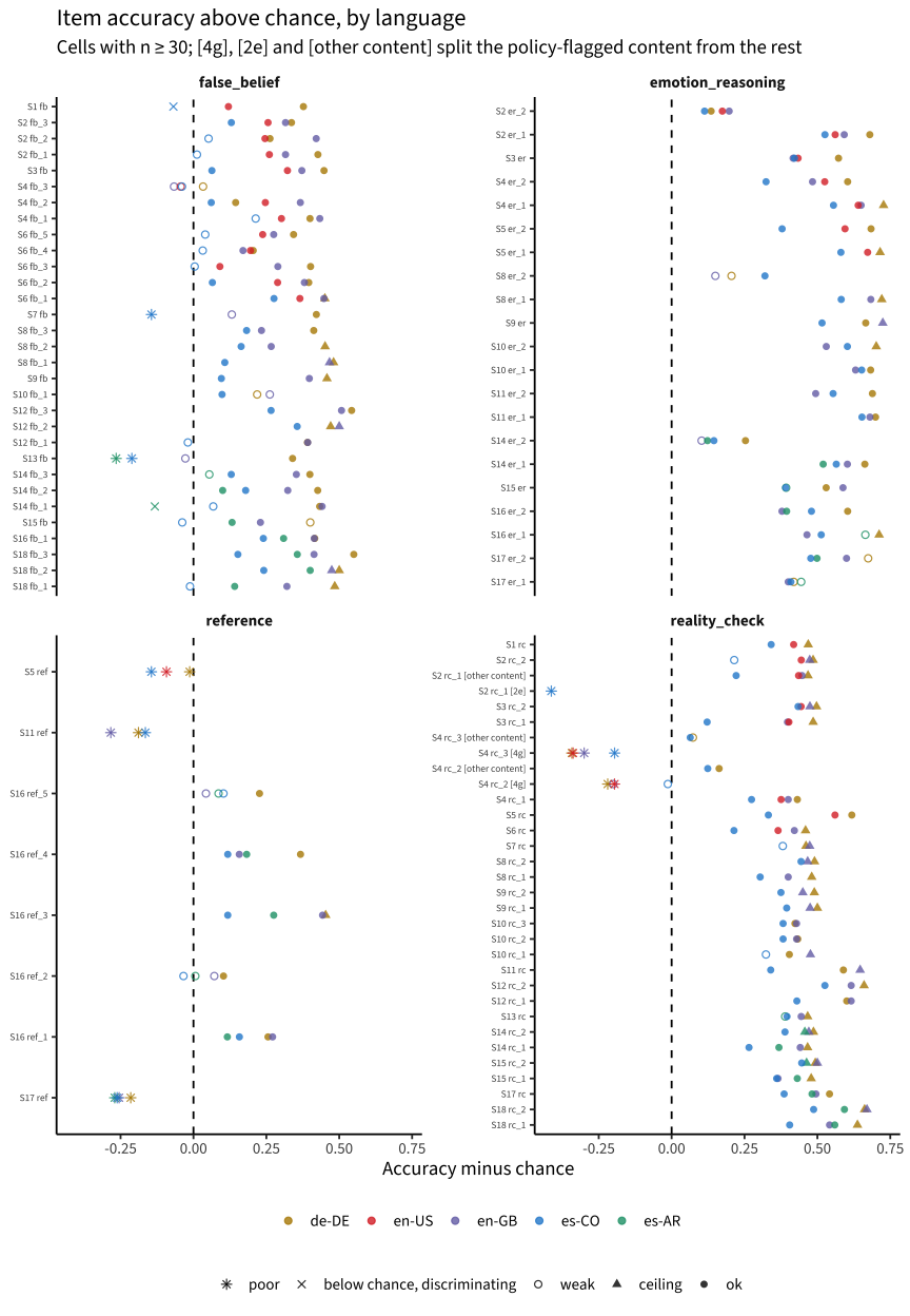
June source Claim June (quoted) Now (2026-09 data) Status
stories_tom §2 Story-construct schemes explain little item difficulty; question type dominates R² ≈ .07–.11 (schemes) question type R² .30; old group .07; new construct .08 survives
stories_tom §2 False-belief targets carry the age signal; controls are flat boxplot; schemes R² ≈ .06 (n.s.) for age above the guessing floor, FB .397 vs controls .276 logit/yr (difference .14 [.04, .24]); raw logit slopes .236 vs .216 (difference .00 [-.07, .07]); 2PL slopes 1.20 vs .85 survives on the chance-corrected scale (raw logit slopes do not separate them; controls also flat because at ceiling)
stories_tom §3 Controls correlate moderately with targets, weakly with age r = .46 and .27 (pooled) pooled .48 / .22; within dataset × form .34 / .13 survives with changes (pooled r reproduces; within a site it is lower)
stories_tom §3 Controls do not gate target age sensitivity similar target~age slopes after pass and fail June method .088 vs .106/SD; GLMM interaction de-DE .23 (p < .0001), en-US .14 (p = .010), es-CO -.04 (p = .21) partly overturned (gating in de-DE and en-US, not in es-CO; descriptive)
stories_tom §3 Dropping controls lowers reliability; keep them marginal .92 → .89 June method .922 → .893; empirical Leipzig .651 → .625; UTDT .669 → .591 survives with changes (direction holds; the magnitudes were model-implied)
stories_tom §5; tom_dimensionality §1 Not cleanly unidimensional ev1/ev2 ≈ 1.9 (Leipzig) Leipzig 1.90; Western/Bogotá/es-AR 2.99–3.25; ECV .59–.73, omega-h/omega-t .93–.97 survives with changes (Leipzig and es-AR; one score defensible elsewhere)
tom_dimensionality §1 Parallel analysis’s 11 factors are over-extraction 11 factors June method 8–13 factors; resampled 1–4 components, 2–10 factors survives (parallel analysis is uninformative here either way)
tom_dimensionality §2 Question type organizes covariance; story weakly; constructs not at all within − between: .101 / .039 / .045 (table) tetrachoric: question type .039–.068; story .005–.027; construct -.028 to .030. Q3 residuals: question type .006–.056, story .015–.040 partly overturned (the tetrachoric pattern reproduces but partly reflects shared difficulty; on Q3 residuals question type groups items only in some samples)
tom_dimensionality §2 Two-factor EFA gives no clean sub-construct factor r .19, 28% variance factor r .21–.39; second factor differs by sample survives
tom_dimensionality §3 A false-belief-only scale is less reliable and no more age-valid Rasch rxx .605 vs .842; age r .401 vs .402 Leipzig alpha .637 vs .675; es-AR age r .354 vs .455 survives
tom_dimensionality synthesis ToM is a reliable composite reliability .92 the .92 is model-implied for a 58-item pool (.922); empirical .554; single fixed forms .36–.82; fCAT .30–.65 overturned
tom_dimensionality synthesis Inter-item correlations are uniformly low ≈ .13 June-style rebuild .129; cleaned .165–.245 survives with changes
tom_dimensionality caveat Story testlet effect is real but weak; a bifactor model is risky not fitted story bifactor better by AIC in all samples; information overstated 13%–23%; θ r .955–.990 new (confirms ‘weak’)
tom_dif_multigroup Scalar invariance is rejected with controls in χ²/df ≈ 29; BIC prefers configural by ≈ 580 release-equivalent June design 30.6, dBIC 626; corrected June design dBIC 249; A χ²/df 7.2, Rasch dBIC 7, 2PL dBIC -68, floor-0 rule dBIC 96; B χ²/df 13.7, dBIC 168 / 87 partly overturned (holds in June’s design and in stories 13–18; in stories 1–6 BIC rejects only under the floor-0 guessing rule)
tom_dif_multigroup; stories_tom §4 Controls are the dominant source of cross-language non-invariance mean |DIF| ≈ 1.9 (controls) vs ≈ 0.5 (targets) release-equivalent 2.01 vs .55; corrected June design 1.43 vs .68; A Rasch 1.74 vs 1.25, 2PL 1.75 vs 1.22; B Rasch .44 vs .86, 2PL 1.03 vs .81 partly overturned (model- and design-dependent; the gap shrank)
tom_dif_multigroup Targets are comparable; false-belief and emotion DIF is small mean |DIF| ≈ 0.5 false belief flagged 6/13 (A), 5/8 (B); story 13 FB es-AR .235; within es-AR across sites 6/29 items flagged overturned (but language is confounded with age, exposure and site)
tom_dif_multigroup Partial scalar invariance is achievable p ≈ .8 (targets) A p = .16 (15 anchors); B p = .36 (20 anchors); without V0 p = .0002 survives descriptively (anchors chosen on the same data; rejected without V0)
tom_dif_multigroup The invariant anchors are mostly false-belief and emotion targets anchor set of targets anchors include 4/7 controls (A) and 6/7 (B); DIF below ≈ 1.3 logits is not detectable survives with changes
tom_reality_check_bug The 4 provable defects are inverted keys (CO moral rc_1, CO reference, late-DE deception rc_2/3) below chance, site-specific story 2 rc_1 .087 on V0 2e only (cause undetermined); story 4 rc_2/3 .328/.188 on image 4g (rc_3 below chance in every language, rc_2 in de-DE and en-US; the key conflicts with the image; flipped r .09/.12); reference .246/.135/.066, below chance except German story 5 (design) partly overturned (the cells are broken, but not site-specific and not all key inversions)
tom_reality_check_bug Repairing the defects removes ≈ 70% of scalar non-invariance χ² 702 → 212 797 → 407 (-49%); controls -77%; PR #27 alone +29% different mechanism (about half, from exclusions, not key flips)
tom_reality_check_bug; README The 12 hand-flagged items are essentially a complete catalog of defects all 12 map onto defects 20 of 28 story-level items un-excluded; 4 keep; 3 scoped; 1 held for the translation check overturned
stories_tom §1 Fixing the scoring bug raised Leipzig test–retest ≈ .45 → ≈ .53 first two runs .487 (released .499; release-equivalent refit .531); 60–180 d .50; > 300 d .30 not replicated (the corrections do not raise it; alternate forms, months apart)
stories_tom §6 Parallel retest items are broadly similar in difficulty within-family SD ≈ 0.9 vs 2.3 not re-tested not re-tested

Synthesis and recommendations

Code
fb_flag <- res_inv$dif |>
  filter(analysis %in% c("A", "B"), question_type == "false_belief", class != "A") |>
  mutate(story = as.integer(str_extract(short, "(?<=story)\\d+"))) |>
  arrange(story) |> pull(short) |> unique()
k$fb_flag_list <- paste(uid_label(fb_flag), collapse = ", ")

Exclusions and corrections (DCC).

  1. Keep item exclusions in the Airtable table, as the DCC prefers, but fix what is there. The 12 generic rows do nothing today (the anti_join runs after recode_tom()), and they would over-exclude if they worked. Replace them with story-level rows: un-exclude the 20 story-level items that behave normally (1 of them weak); exclude reference_reference in stories 5/11/17 and story 10’s deception false belief 1 everywhere; and add the three content-scoped rows above, which need a content-version (or date-window) column. Hold any Spanish row for story 13 until the translation check. Every row, with its exact scope, trial count and rationale, is listed in All recommended item actions.
  2. The same reasoning applies to corrections. PR #27 writes its identity remaps (fix_tom_item_uids(): a 25-row table keyed on date window, item code, answer and occurrence) and three per-story chance values into levantemodels code. Those are data properties too. A metadata table, such as the item-mapping tables in levante_metadata_items, would document them next to the exclusions, and could also hold a scoped key correction for the story-4 reality checks on image 4g if the content team confirms that “no” is right for that scene (that would keep 1,243 trials). This is a design choice for the DCC; the analysis only needs the corrections applied somewhere.
  3. Consider V0 Bogotá story-2 reality check 2 and story 5’s reference reality check (non-invariant only because of V0) as further V0-scoped rows, next to V0 reality check 1, whose cause stays undetermined. For reality check 2 the monotonicity screen supports this: on the V0 scene higher scorers do worse (see Do higher scorers do better?).

Deployed items (core-tasks; item bank).

  1. Re-author story-4 reality checks 2/3 for image 4g (or change their key, as above), and redesign reference_reference (stories 5/11/17; see The reference questions). Both are still in the deployed corpora.
  2. Exclude or rewrite story 17’s emotion reasoning 1 (“How do you think Mom feels about not finding the book she wanted?”): it is flat overall and reversed in German, where higher scorers answer surprised. Review the near-chance yes/no “Is [sibling] mad at [sibling]?” questions (story 4 fb_3, story 16 ref_2) and story 10’s deception false belief 1, and the same-scene doublets (story 6 fb_2/fb_5, both keyed “shoes”; story 4 fb_2/fb_3, both “no”).
  3. Check the Spanish translations (es-CO, es-AR) of the false-belief prompts: every false-belief item flagged (class B or C) in the invariance analyses (S1 fb, S2 fb_1, S2 fb_2, S3 fb, S4 fb_2, S6 fb_3, S13 fb, S14 fb_1, S14 fb_2, S14 fb_3, S18 fb_1), plus story 7’s reality_known item, which the item screen flags (stories 7–12 are in no invariance analysis). Translation is one hypothesis; prior exposure to the task and the samples themselves are others. (Sites that share a language differ less and on other items, and the false-belief DIF persists with younger German children, so site and age alone do not explain it.) Until the check is done, keep the Spanish sensitivity flag and report results with and without it; it changes scores very little.

Scoring.

  1. Score group by group (the PR #26 rule, not yet merged). Before changing production’s integration grid, investigate how the low-scoring groups’ means and variances depend on the grid, the latent density and the guessing convention: all three move them, while scores within a group barely change. For the RfP1 datasets that v2_3 scored under the German prior, their own prior alone lowers the level by .5–2.5 logits (.5–2.6 in total).
  2. Recalibrate ToM on the current data once PR #27 is merged. The analysis model here uses 3,079 runs in 8 groups. The 2PL is preferred, and local dependence is modest, so a testlet model is optional. If it is skipped, discount story information by about 13%–23% in reliability claims. The block-CAT simulation shows it does not change which stories are selected.
  3. Treat cross-language comparisons of Stories scores as partial-scalar at best, and remember that the language groups also differ in age, prior exposure and site. Report group differences only with that caveat and adjusted for age.

Block CAT and the item bank.

  1. The deployed fCAT is a random 3-story form with reliability .30–.65 in a median of 4.4–5.6 minutes. In the same children, three random stories instead of a six-story form cost .11–.19 in reliability for half the time. The 3-vs-4 decision is mostly a trade of minutes for precision; the simulation in Designing the block CAT recommends 4 stories (today’s blocks plus one free story) with adaptive selection.
  2. Adaptive selection within blocks helps: choosing the more informative of the form’s two stories per block raises the reliability of a 3-story form by a median of .05 (up to .12) in the same time. With six stories per block it does more (simulation: .51 → .63), but the bank is thin above θ = 0 on the DE scale, so real gains also need harder stories and items, calibrated in several languages. The fCAT’s fixed block order confounds block with position; randomize it if blocks are to be compared.
  3. The block structure need not follow the story constructs, which do not organize the item covariance. Question type’s tetrachoric clustering partly reflects shared difficulty; once difficulty and guessing are modelled, what remains is weak and uneven across samples. Blocks can be chosen for content coverage and time.
  4. Keep scoring the controls. If time binds, they are the least informative questions per item. Whether to keep administering them as comprehension checks is a design decision; the data show that a failed control makes the story’s targets less age-informative mainly in Leipzig (and to a lesser degree in en-US), not in es-CO.
  5. Only Leipzig has repeat data, as alternate forms months apart. A short-interval retest (same or parallel forms, about 2 weeks) at a high-volume site would give the first real test–retest estimate.

Methods notes and caveats

  • Post-hoc rules. Two rules in the items analysis were revised after its first run and are disclosed in res_items$meta$notes: the weak-item flag and the age-slope minority rule. The originals are kept in r_ir_below_10 and age_slope_raw. The 2026-09 revision added, after review: the floor-corrected age slopes with a symmetric filter, the flipped-key check, the per-language discrimination rule for the Spanish items, story 10’s deception false belief 1 as a policy exclusion, the within-language and age-restricted invariance variants, the 2PL tests, the latent-density check and the block-CAT simulation.
  • Guessing floor. The reliability and invariance models fix it at chance; the dimensionality models set it to 0 for items answered at or below chance in the sample. The invariance and reliability conclusions were rechecked under the dimensionality rule (A_g0/B_g0 and the g0 sensitivity of the reliability model). Neither rule can represent a group that answers systematically below chance, as young children do on reality_known false-belief questions.
  • mirt::marginal_rxx() integrates TI/(TI + var) over N(0, 1) and assumes every item in the matrix is answered. The June chapters’ “.92”, “.89” and “.84” come from it on sparse, multi-form matrices. This chapter reports empirical reliability instead.
  • MAP, not ML. The fixed-floor 2PL and bifactor fits in the dimensionality analysis use an N(0, 2²) slope prior, and the invariance 2PL uses the production priors; their AIC and BIC are evaluated at MAP estimates. The bootstrap intervals for ev1/ev2 are biased downward, so the chapter reports a bootstrap SE instead of percentile intervals.
  • Upper bounds. The reliabilities come from unidimensional models that assume scalar invariance, so they overstate precision somewhat (footnote in the reliability section).
  • Confounds. Language, site, age, prior exposure, form and deployment epoch overlap. The es-AR samples are young (4.8–8.4 years), the Leipzig samples are older, near ceiling and mostly on repeat runs in stories 13–18, and es-CO in the invariance analysis pools 4 datasets from 2024–2026. The age-band plots describe; they are not a model-based age adjustment.
  • Coverage. en-GB (Sheffield, fCAT only) has too few responses per item for the invariance analyses. en-US items from stories 7–18 have fewer than 30 responses. Stories 7–12 are sparse everywhere.
  • Gating conditions on passing a control, which depends on ability, so it is descriptive.
  • Invariance fits use mirt’s default θ range (see the numerics note).
  • Not re-tested: June’s parallel-retest-family analysis (stories_tom §6).

Reproducing

The chapter reads only cached files in data/stories_2026-09/ (gitignored) and fits no models. To rebuild, run the scripts in the order below with Rscript from a working directory outside the repo (the book’s renv has an mgcv binary that breaks mirt). Each script takes the book root as its argument (else STORIES_BOOK_ROOT, else the directory above the script’s tasks/ folder). The build must come first; the four analysis scripts only read its output and can run in any order after it.

Code
tribble(
  ~step, ~script, ~writes, ~built,
  1, "tasks/_build_stories_data.R", "stories_trials.rds, stories_runs.rds, reconciliation.rds, README.md (and, if missing, the pinned raw pulls, release snapshots and the v2_3 model record)", format(prov$built_at),
  2, "tasks/_stories_fits_items.R", "results_items.rds", format(res_items$meta$built_at),
  3, "tasks/_stories_fits_dimensionality.R", "results_dimensionality.rds",
  paste0(res_dim$meta$run_at, " (", round(as.numeric(difftime(as.POSIXct(res_dim$meta$finished_at), as.POSIXct(res_dim$meta$run_at), units = "mins")), 1), " min)"),
  4, "tasks/_stories_fits_invariance.R", "results_invariance.rds",
  paste0(res_inv$meta$created, " (", round(res_inv$meta$runtime_min, 1), " min)"),
  5, "tasks/_stories_fits_reliability.R", "results_reliability.rds, stories_scores_analysis.rds", format(res_rel$meta$built_at)
) |>
  knitr::kable(caption = "Scripts in run order, outputs and build times")
Scripts in run order, outputs and build times
step script writes built
1 tasks/_build_stories_data.R stories_trials.rds, stories_runs.rds, reconciliation.rds, README.md (and, if missing, the pinned raw pulls, release snapshots and the v2_3 model record) 2026-09-24 23:04:31
2 tasks/_stories_fits_items.R results_items.rds 2026-09-24 23:20:55
3 tasks/_stories_fits_dimensionality.R results_dimensionality.rds 2026-09-24 23:21:16.702636 (15.8 min)
4 tasks/_stories_fits_invariance.R results_invariance.rds 2026-09-24 23:46:13.961093 (14.7 min)
5 tasks/_stories_fits_reliability.R results_reliability.rds, stories_scores_analysis.rds 2026-09-24 23:41:44
cd /some/dir/outside/the/repo
export LEVANTEMODELS_PATH=/path/to/levantemodels   # checkout of PR #27's branch
Rscript /path/to/levante-analysis/tasks/_build_stories_data.R /path/to/levante-analysis
Rscript /path/to/levante-analysis/tasks/_stories_fits_items.R /path/to/levante-analysis
Rscript /path/to/levante-analysis/tasks/_stories_fits_dimensionality.R /path/to/levante-analysis
STORIES_CORES=6 Rscript /path/to/levante-analysis/tasks/_stories_fits_invariance.R /path/to/levante-analysis
Rscript /path/to/levante-analysis/tasks/_stories_fits_reliability.R /path/to/levante-analysis

The data build and the reliability script load levantemodels from the PR #27 source tree with pkgload::load_all(). LEVANTEMODELS_PATH must point to a checkout of branch fix-tom-identity-corrections (they stop if it is unset). They record its commit (3dc148b for the reliability run). Every results file’s meta element records the inputs, thresholds, package versions and sessionInfo(). The data build pins every raw dataset version (table above); the release snapshots are pinned by processed version, except Sheffield’s unreleased next draft, which cannot be pinned.


  1. The flag rules were revised once after the first run. The original weak-item rule (item-rest r point estimate < .10) mostly flagged small fCAT cells, whose item-rest CIs are wide. The revised rule uses the CI upper bound, checks ceiling before weak, and gives below-chance items with a credibly positive r their own level. The original criterion is kept in r_ir_below_10; it would flag 86 of the 327 cells.↩︎

  2. The classes were revised once after the first run, which had a single “no credible gain” class for every CI that included 0. That class mixed items that are flat with precision (story 17’s emotion reasoning 1, n = 1,374) with small fCAT-only items whose CIs are wide, so it was split at a gain of .10. The screen by content version was also added after the first run, because story 2’s reality check 2 was flat overall but reversed on one scene.↩︎

  3. The minority rule (≥ 10 correct and ≥ 10 incorrect) was added after the first run, where one near-ceiling item gave a separated slope of −170. That slope dominated the R² values. Because of the rule, control slopes come only from samples where controls are not at ceiling. Unfiltered slopes are kept in age_slope_raw.↩︎

  4. Both assumptions make them upper bounds. The dimensionality analysis finds that the unidimensional model overstates test information by 13%–23%, which lowers reliability by .015–.039 in its samples; and scalar invariance does not fully hold (see the invariance section).↩︎