10 — Downward extension (Boston Children’s, ages 2–5): hand scores, official scores, and task selection
ImportantAI-generated — not for publication
The code and prose in this chapter were written by Claude Code (an AI coding agent) under human direction. They have not been line-by-line verified by a human and must not be published or cited as-is.
WarningPreliminary & unvetted analysis
These are exploratory analyses of preliminary, in-progress LEVANTE data. Results have not been reviewed or validated and require checking by the LEVANTE Data Coordinating Center before any use.
Purpose
Downward-extension data from Boston Children’s Hospital (Nelson site) — children aged 2–5, piloting the LEVANTE core tasks below the 5–12 range they were built for. Updated 2026-08-31: the sample has grown to 44 children / 378 runs (from 31/228 in the first June–August tranche), with collection through Aug 29. There are still no validated scoring models for this age band, so hand-scoring uses the raw per-site dataset (pilot_bostonchildrens_us_main_raw:7e6c, pinned to v5_0), not levante_data_latest.
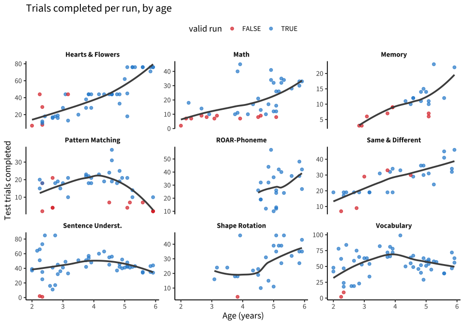
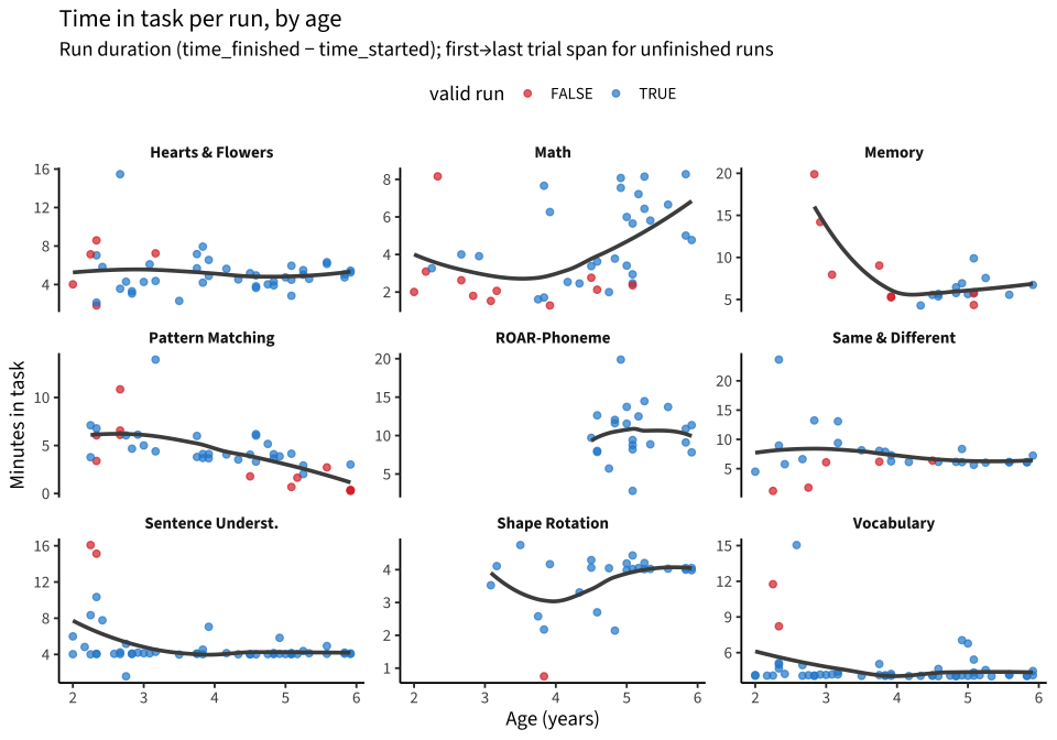
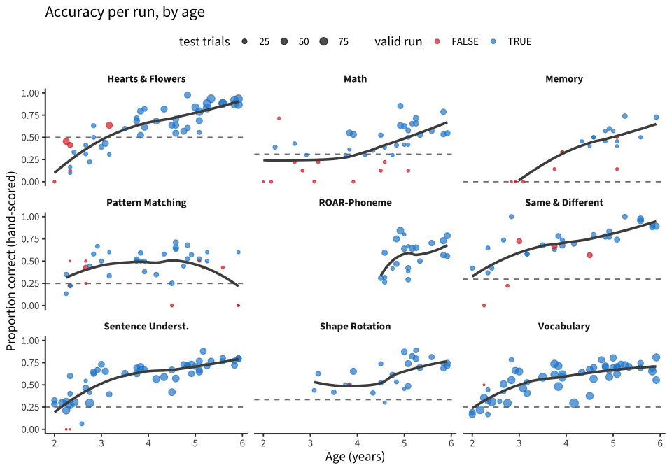
Two aims: (A) hand-score the tasks from trial-level correctness with simple, transparent rules; (B) describe accuracy, time in task, and trials completed across tasks and ages. Along the way we log data-quality flags — this is a pilot, so what breaks is as informative as what works.
Code
source(here::here("common.R"))library(tidyverse)library(patchwork)DS_REF <-"pilot_bostonchildrens_us_main_raw:7e6c"DS_VER <-"v5_0"# Raw tables are cached to data/ (git-ignored); pull via levante::get_raw_table()# if a cache is missing. Pinned to DS_VER for reproducibility.load_raw <-function(table) { path <-here("data", glue("downex_boston_{table}_{DS_VER}.rds"))if (!file_exists(path)) {dir_create(here("data"))write_rds(levante::get_raw_table(table, data_source = DS_REF,data_source_version = DS_VER), path) }read_rds(path)}users <-load_raw("users")runs <-load_raw("runs") |>filter(task_id !="schema_row")trials <-load_raw("trials") |>filter(task_id !="schema_row")variants <-load_raw("variants") |>filter(task_id !="schema_row")task_labels <-c(`hearts-and-flowers`="Hearts & Flowers", `memory-game`="Memory",`same-different-selection`="Same & Different", `matrix-reasoning`="Pattern Matching",`mental-rotation`="Shape Rotation", `egma-math`="Math", vocab ="Vocabulary",trog ="Sentence Underst.", pa ="ROAR-Phoneme")
1. Who and what: the sample and the runs
Ages come from birth_month/birth_year and each run’s time_started (month precision). Only children (user_type == "student") are kept.
Code
kids <- users |>filter(user_type =="student") |>select(user_id, birth_month, birth_year, sex)runs <- runs |>inner_join(kids, by ="user_id") |>mutate(task = task_labels[task_id],age = (year(time_started) - birth_year) + (month(time_started) - birth_month) /12,age_yr =floor(age),# time in task: run duration if finished, else first→last trial timestampdur_min =as.numeric(difftime(time_finished, time_started, units ="mins")))trial_span <- trials |>group_by(run_id) |>summarise(span_min =as.numeric(difftime(max(server_timestamp), min(server_timestamp), units ="mins")), .groups ="drop")runs <- runs |>left_join(trial_span, by ="run_id") |>mutate(dur_min =coalesce(dur_min, span_min))kids_age <- runs |>group_by(user_id, sex) |>summarise(age =min(age), .groups ="drop") |>mutate(age_yr =floor(age))kids_age |>count(age_yr, sex) |>pivot_wider(names_from = sex, values_from = n, values_fill =0) |>mutate(total =rowSums(across(-age_yr))) |> knitr::kable(caption =glue("Children by age (years) at first run — N = {nrow(kids_age)}"))
Children by age (years) at first run — N = 44
age_yr
NA
total
2
16
16
3
6
6
4
10
10
5
12
12
Code
runs |>group_by(task) |>summarise(runs =n(), children =n_distinct(user_id), completed =sum(completed),valid =sum(valid_run), adaptive =any(variant_id %in% variants$variant_id[variants$adaptive]),.groups ="drop") |>arrange(desc(runs)) |> knitr::kable(caption ="Runs per task (completed = dashboard flag; valid = passes the pipeline's run validation)")
Runs per task (completed = dashboard flag; valid = passes the pipeline’s run validation)
task
runs
children
completed
valid
adaptive
Vocabulary
62
44
58
51
TRUE
Sentence Underst.
52
41
50
49
TRUE
Hearts & Flowers
50
36
46
40
FALSE
Pattern Matching
50
30
38
29
TRUE
Math
42
33
37
28
TRUE
ROAR-Phoneme
33
19
20
22
FALSE
Shape Rotation
32
24
28
25
TRUE
Same & Different
31
25
29
25
TRUE
Memory
26
22
22
13
FALSE
Code
runs |>count(completed, valid_run, validation_msg_run) |>arrange(desc(n)) |> knitr::kable(caption ="Run validity flags. `less_than_10_test_trials` is the pipeline's minimum-length rule.")
Run validity flags. less_than_10_test_trials is the pipeline’s minimum-length rule.
completed
valid_run
validation_msg_run
n
TRUE
TRUE
NA
275
TRUE
FALSE
less_than_10_test_trials
45
FALSE
FALSE
less_than_10_test_trials
43
TRUE
FALSE
straightlining_10
8
FALSE
TRUE
NA
7
Most runs are complete and valid, but a sizeable minority end with fewer than 10 test trials — the pipeline’s validity floor. Where in the age range those short runs sit is one of the first things to check (§3).
2. Trial-level prep and hand-scoring rules
We keep test trials only (is_practice_trial == FALSE), and apply minimal, task-specific rules that mirror what levantemodels::recode_trials() does for the released data:
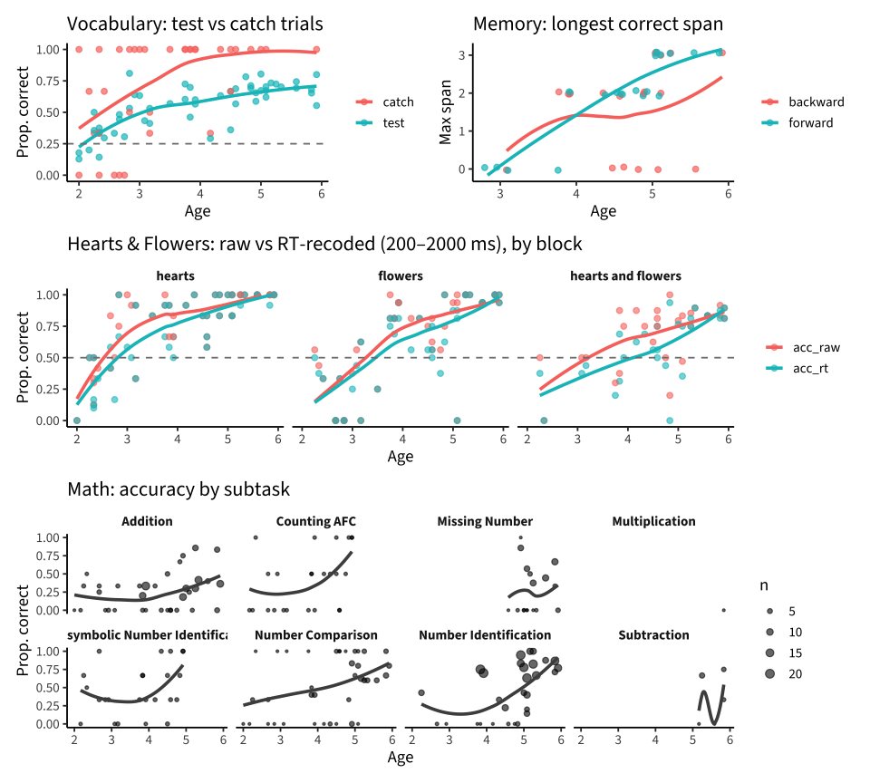
Hearts & Flowers: a response is correct only if 200 ms ≤ RT ≤ 2000 ms (too-fast/too-slow → incorrect); we report raw accuracy too. Blocks are hearts / flowers / hearts and flowers (mixed).
Vocabulary: catch trials (attention checks) are scored separately from test trials.
Memory (Corsi): span score = the longest sequence length answered correctly, forward and backward.
Math: accuracy overall and by subtask (corpus_trial_type).
Chance per trial is derived from the recorded distractors field (chance = 1 / (n distractors + 1)); Hearts & Flowers is 2-AFC by design; Memory is free recall (chance 0); ROAR-Phoneme records no distractors (chance left NA).
Everything else: proportion correct on test trials.
Per task × age-year: runs, share valid, median trials, median minutes, mean accuracy
task
runs_2y
runs_3y
runs_4y
runs_5y
pct_valid_2y
pct_valid_3y
pct_valid_4y
pct_valid_5y
trials_2y
trials_3y
trials_4y
trials_5y
minutes_2y
minutes_3y
minutes_4y
minutes_5y
acc_2y
acc_3y
acc_4y
acc_5y
Hearts & Flowers
12
11
9
13
0.67
0.91
1.00
1.00
16.5
38
44.0
76.0
4.2
5.7
4.3
5.1
0.31
0.59
0.69
0.84
Math
8
7
10
14
0.38
0.57
0.80
0.93
8.5
10
15.0
29.0
3.2
1.7
3.1
5.7
0.27
0.28
0.41
0.55
Memory
2
4
7
8
0.00
0.00
1.00
0.75
3.0
8
12.0
11.5
17.0
6.7
5.7
5.8
0.00
0.20
0.50
0.50
Pattern Matching
11
9
11
10
0.55
1.00
0.91
0.40
18.0
21
21.0
7.0
6.1
4.1
4.1
1.8
0.39
0.49
0.49
0.36
ROAR-Phoneme
NA
NA
8
14
NA
NA
1.00
1.00
NA
NA
29.0
31.5
NA
NA
10.7
10.1
NA
NA
0.49
0.60
Same & Different
8
9
6
7
0.75
0.78
0.83
1.00
19.0
29
31.5
34.0
6.2
7.9
6.2
6.1
0.48
0.67
0.74
0.91
Sentence Underst.
19
9
10
13
0.89
1.00
1.00
1.00
37.0
49
49.0
42.0
4.2
4.1
4.0
4.1
0.35
0.64
0.63
0.75
Shape Rotation
NA
7
6
13
NA
0.86
1.00
1.00
NA
18
20.5
35.0
NA
3.5
3.7
4.0
NA
0.52
0.52
0.73
Vocabulary
17
11
11
14
0.88
1.00
1.00
1.00
47.0
66
52.0
56.5
4.2
4.1
4.1
4.1
0.38
0.58
0.61
0.70
4. Hand scores per task
4.1 Sanity check: hand accuracy vs the dashboard’s own count
The runs table carries the dashboard’s num_correct/num_attempted. Our hand-scored accuracy should agree except where our rules deliberately differ (H&F RT recode; vocab catch trials excluded).
Code
run_sum |>filter(!is.na(num_attempted), num_attempted >0) |>mutate(dash_acc = num_correct / num_attempted) |>group_by(task) |>summarise(runs =n(), r =cor(acc_raw, dash_acc, use ="complete.obs"),mean_diff =mean(acc_raw - dash_acc, na.rm =TRUE),trials_match =mean(n_trials == num_attempted), .groups ="drop") |> knitr::kable(digits =2, caption ="Raw hand accuracy vs dashboard num_correct/num_attempted (r, mean difference, share of runs with identical trial counts)")
Raw hand accuracy vs dashboard num_correct/num_attempted (r, mean difference, share of runs with identical trial counts)
task
runs
r
mean_diff
trials_match
Hearts & Flowers
45
1.00
0.00
1.00
Math
39
1.00
0.00
1.00
Memory
21
1.00
0.23
0.00
Pattern Matching
41
1.00
0.00
1.00
ROAR-Phoneme
22
1.00
0.00
1.00
Same & Different
30
0.89
-0.01
0.07
Sentence Underst.
51
1.00
0.00
1.00
Shape Rotation
26
1.00
0.00
1.00
Vocabulary
53
1.00
0.00
1.00
Where the two are directly comparable (Shape Rotation, ROAR-Phoneme, Sentence Understanding, Vocabulary) the hand score reproduces the dashboard count exactly (r = 1, identical trial counts). Memory and Same & Different count “trials” differently (sequences / multi-response stages), so they don’t match by construction; the remaining tasks have some runs with no dashboard count.
4.2 Task-specific scores
Code
# Vocabulary: test vs catchvocab_h <- test |>filter(task_id =="vocab") |>group_by(run_id, user_id, age, kind = corpus_trial_type) |>summarise(n =n(), acc =mean(correct), .groups ="drop")# Hearts & Flowers: raw vs RT-recoded, by blockhf_h <- test |>filter(task_id =="hearts-and-flowers") |>group_by(run_id, user_id, age, block = corpus_trial_type) |>summarise(n =n(), acc_raw =mean(correct), acc_rt =mean(correct_hand),med_rt =median(rt_numeric, na.rm =TRUE), .groups ="drop") |>mutate(block =factor(block, c("hearts", "flowers", "hearts and flowers")))# Memory: longest correct span, forward / backwardmem_h <- test |>filter(task_id =="memory-game") |>separate(corpus_trial_type, into =c("direction", "span"), sep ="-", convert =TRUE) |>group_by(run_id, user_id, age, direction) |>summarise(n =n(), max_span =if (any(correct)) max(span[correct]) else0, .groups ="drop")# Math: by subtaskmath_h <- test |>filter(task_id =="egma-math") |>group_by(run_id, user_id, age, subtask = corpus_trial_type) |>summarise(n =n(), acc =mean(correct), chance =mean(chance), .groups ="drop")# Same & Different: by trial typesds_h <- test |>filter(task_id =="same-different-selection") |>group_by(run_id, user_id, age, type = corpus_trial_type) |>summarise(n =n(), acc =mean(correct), .groups ="drop")
Code
p_vocab <-ggplot(vocab_h, aes(age, acc, colour = kind)) +geom_point(alpha =0.7) +geom_smooth(method ="loess", se =FALSE, span =1) +geom_hline(yintercept =0.25, linetype ="dashed", colour ="grey50") +ylim(0, 1) +labs(title ="Vocabulary: test vs catch trials", x ="Age", y ="Prop. correct", colour =NULL)p_hf <- hf_h |>pivot_longer(c(acc_raw, acc_rt), names_to ="scoring", values_to ="acc") |>ggplot(aes(age, acc, colour = scoring)) +geom_point(alpha =0.6) +geom_smooth(method ="loess", se =FALSE, span =1) +geom_hline(yintercept =0.5, linetype ="dashed", colour ="grey50") +facet_wrap(~block) +ylim(0, 1) +labs(title ="Hearts & Flowers: raw vs RT-recoded (200–2000 ms), by block", x ="Age", y ="Prop. correct", colour =NULL)p_mem <-ggplot(mem_h, aes(age, max_span, colour = direction)) +geom_jitter(width =0.05, height =0.08, alpha =0.7) +geom_smooth(method ="loess", se =FALSE, span =1) +labs(title ="Memory: longest correct span", x ="Age", y ="Max span", colour =NULL)p_math <-ggplot(math_h, aes(age, acc)) +geom_point(alpha =0.6, aes(size = n)) +geom_smooth(method ="loess", se =FALSE, span =1.2, colour ="grey30") +facet_wrap(~subtask, nrow =2) +ylim(0, 1) +scale_size_area(max_size =3) +labs(title ="Math: accuracy by subtask", x ="Age", y ="Prop. correct")(p_vocab + p_mem) / p_hf / p_math +plot_layout(heights =c(1, 1, 1.4))
Hand scores by task component × age year (mean over runs)
task
part
n_runs_2y
n_runs_3y
n_runs_4y
n_runs_5y
score_2y
score_3y
score_4y
score_5y
Hearts & Flowers
flowers
8
11
9
13
0.19
0.58
0.64
0.88
Hearts & Flowers
hearts
12
11
9
13
0.38
0.67
0.85
0.96
Hearts & Flowers
hearts and flowers
2
6
9
12
0.19
0.42
0.56
0.78
Math
Addition
8
7
10
10
0.18
0.17
0.24
0.37
Math
Counting AFC
7
7
10
NA
0.29
0.29
0.60
NA
Math
Missing Number
NA
NA
4
13
NA
NA
0.46
0.22
Math
Multiplication
NA
NA
NA
1
NA
NA
NA
0.00
Math
Non-symbolic Number Identification
7
7
10
NA
0.45
0.29
0.63
NA
Math
Number Comparison
8
7
10
13
0.33
0.47
0.52
0.72
Math
Number Identification
3
4
8
14
0.14
0.36
0.29
0.66
Math
Subtraction
NA
NA
NA
5
NA
NA
NA
0.35
Memory (max span)
backward
NA
4
7
7
NA
1.50
1.14
2.00
Memory (max span)
forward
2
4
7
8
0.00
1.00
2.00
2.88
Pattern Matching
all
11
9
11
10
0.39
0.49
0.49
0.36
ROAR-Phoneme
all
NA
NA
8
14
NA
NA
0.49
0.60
Same & Different
2-match
NA
1
3
7
NA
0.50
0.56
0.84
Same & Different
3-match
NA
NA
NA
3
NA
NA
NA
0.88
Same & Different
4-match
NA
3
2
2
NA
0.28
0.88
0.45
Same & Different
instructions
NA
4
5
7
NA
0.50
0.60
1.00
Same & Different
something-same-1
NA
5
6
NA
NA
0.00
0.00
NA
Same & Different
something-same-2
NA
5
5
NA
NA
0.64
0.88
NA
Same & Different
test-dimensions
8
9
6
7
0.48
0.81
0.96
0.99
Sentence Underst.
all
19
9
10
13
0.35
0.64
0.63
0.75
Shape Rotation
all
NA
7
6
13
NA
0.52
0.52
0.73
Vocabulary
catch
15
11
6
3
0.50
0.89
0.83
1.00
Vocabulary
test
17
11
11
14
0.38
0.57
0.60
0.70
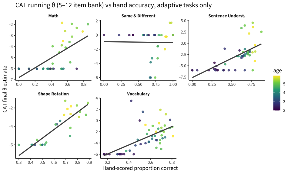
4.3 The CAT’s running θ as an (unvalidated) provisional score
Several tasks ran as adaptive variants, so each trial carries the CAT’s running theta_estimate on the 5–12 calibrated item bank. That bank is out of range for 2–5-year-olds (see the flags below), so this is not a score to use — but its relation to hand accuracy tells us whether the CAT is discriminating at all down here.
Code
theta_last <- test |>filter(!is.na(theta_estimate)) |>group_by(run_id) |>slice_max(trial_index, n =1, with_ties =FALSE) |>select(run_id, theta_last = theta_estimate) |>inner_join(run_sum, by ="run_id") |>group_by(task) |>filter(n() >=5) |>ungroup() # drop tasks with a handful of CAT runsggplot(theta_last, aes(acc, theta_last)) +geom_point(aes(colour = age), alpha =0.8) +geom_smooth(method ="lm", se =FALSE, colour ="grey30") +facet_wrap(~task, scales ="free") +scale_colour_viridis_c(name ="age") +labs(x ="Hand-scored proportion correct", y ="CAT final θ estimate",title ="CAT running θ (5–12 item bank) vs hand accuracy, adaptive tasks only")
Code
theta_last |>group_by(task) |>summarise(runs =n(), r_theta_acc =cor(theta_last, acc), r_theta_age =cor(theta_last, age),mean_theta =mean(theta_last), .groups ="drop") |> knitr::kable(digits =2, caption ="Final CAT θ: agreement with hand accuracy and age, and mean level (on the 5–12 scale)")
Final CAT θ: agreement with hand accuracy and age, and mean level (on the 5–12 scale)
task
runs
r_theta_acc
r_theta_age
mean_theta
Math
39
0.68
0.67
-5.00
Same & Different
30
-0.01
-0.09
-1.02
Sentence Underst.
51
0.64
0.68
-2.84
Shape Rotation
26
0.86
0.66
-4.12
Vocabulary
53
0.62
0.49
-3.08
The CAT does discriminate down here on Math, Shape Rotation, Sentence Understanding, and Vocabulary (θ–accuracy r ≈ 0.5–0.85), but the θ values are far below the 5–12 scale (means ≈ −2.7 to −5.2), and a whole row of runs — mostly the 2–3-year-olds — sits at exactly θ = −6, the estimator’s hard lower bound: those are floor codes, not measurements. Same & Different’s θ is unrelated to accuracy (r ≈ 0.1) and many of its runs sit at exactly 0 (the prior mean, i.e. θ never updated), consistent with its scoring being under revision.
4.4 Vocabulary: item-level accuracy
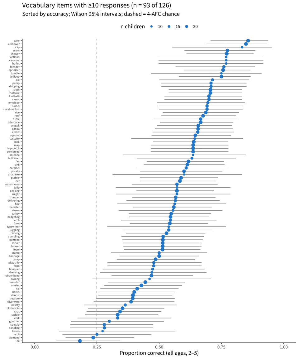
Vocabulary is a CAT, so each child sees a different subset of the 126 items and each item at most once — per-item Ns are small (mostly 10–23) and these estimates are very noisy. Bars are Wilson 95% intervals; the dashed line is 4-AFC chance.
Code
wilson <-function(p, n, z =1.96) { c <- (p + z^2/ (2* n)) / (1+ z^2/ n) h <- z *sqrt(p * (1- p) / n + z^2/ (4* n^2)) / (1+ z^2/ n)tibble(lo =pmax(0, c - h), hi =pmin(1, c + h))}vi <- test |>filter(task_id =="vocab", corpus_trial_type =="test") |>mutate(grp =if_else(age <3, "2-year-olds", "3+"))item_all <- vi |>group_by(item) |>summarise(n =n(), acc =mean(correct), .groups ="drop") |>filter(n >=10) |>mutate(wilson(acc, n)) |>mutate(item =fct_reorder(item, acc))ggplot(item_all, aes(acc, item)) +geom_vline(xintercept =0.25, linetype ="dashed", colour ="grey50") +geom_errorbarh(aes(xmin = lo, xmax = hi), height =0, colour ="grey60") +geom_point(aes(size = n), colour ="#268bd2") +scale_size_area(max_size =3.5, breaks =c(10, 15, 20), name ="n children") +scale_x_continuous(limits =c(0, 1), breaks =seq(0, 1, 0.25)) +labs(x ="Proportion correct (all ages, 2–5)", y =NULL,title =glue("Vocabulary items with ≥10 responses (n = {nrow(item_all)} of 126)"),subtitle ="Sorted by accuracy; Wilson 95% intervals; dashed = 4-AFC chance") +theme(axis.text.y =element_text(size =7), legend.position ="top")
Code
bind_rows(item_all |>slice_max(acc, n =10) |>mutate(end ="easiest"), item_all |>slice_min(acc, n =10) |>mutate(end ="hardest")) |>select(end, item, n, acc, lo, hi) |>mutate(across(c(acc, lo, hi), ~round(.x, 2))) |> knitr::kable(caption ="Ten easiest and ten hardest vocabulary items (≥10 responses), all ages")
Ten easiest and ten hardest vocabulary items (≥10 responses), all ages
end
item
n
acc
lo
hi
easiest
cake
35
0.86
0.71
0.94
easiest
sunflower
33
0.85
0.69
0.93
easiest
ship
12
0.83
0.55
0.95
easiest
acorn
31
0.77
0.60
0.89
easiest
shower
35
0.77
0.61
0.88
easiest
buffet
13
0.77
0.50
0.92
easiest
carousel
13
0.77
0.50
0.92
easiest
wetland
13
0.77
0.50
0.92
easiest
blender
25
0.76
0.57
0.89
easiest
sprinkler
37
0.76
0.60
0.87
hardest
oil
33
0.18
0.09
0.34
hardest
diamond
34
0.24
0.12
0.40
hardest
latch
20
0.25
0.11
0.47
hardest
kazoo
11
0.27
0.10
0.57
hardest
sandbag
25
0.28
0.14
0.48
hardest
spatula
25
0.28
0.14
0.48
hardest
gourmet
20
0.30
0.15
0.52
hardest
cork
21
0.33
0.17
0.55
hardest
saddle
36
0.33
0.20
0.50
hardest
chat
35
0.34
0.21
0.51
The easy end is what you’d expect for preschoolers (sunflower, sprinkler, cake, marshmallow); the hard end mixes genuinely late-acquired words (gourmet, silverware, cork) with a couple sitting below chance (latch 0.15, oil 0.20). Not significant at these Ns (both intervals include 0.25), but below-chance accuracy is the same key/picture-defect signal we use in the 5–12 data — worth a look at those two items’ pictures/distractors.
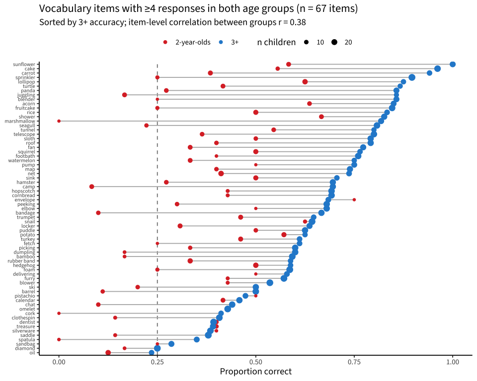
By age — 2-year-olds vs 3+. Only items with ≥4 responses in each group are shown (the 2-year-olds contribute just 688 test trials in total), so the 2-year-old estimates in particular are extremely noisy.
Code
item_age <- vi |>group_by(item, grp) |>summarise(n =n(), acc =mean(correct), .groups ="drop") |>group_by(item) |>filter(n_distinct(grp) ==2, all(n >=4)) |>ungroup()ord_items <- item_age |>filter(grp =="3+") |>arrange(acc) |>pull(item)item_age <- item_age |>mutate(item =factor(item, levels = ord_items))wide <- item_age |>select(item, grp, acc, n) |>pivot_wider(names_from = grp, values_from =c(acc, n))r_age <-cor(wide$`acc_2-year-olds`, wide$`acc_3+`)ggplot(item_age, aes(acc, item)) +geom_vline(xintercept =0.25, linetype ="dashed", colour ="grey50") +geom_line(aes(group = item), colour ="grey70") +geom_point(aes(colour = grp, size = n)) +scale_colour_manual(values =c(`2-year-olds`="#dc322f", `3+`="#268bd2"), name =NULL) +scale_size_area(max_size =4, name ="n children") +scale_x_continuous(limits =c(0, 1), breaks =seq(0, 1, 0.25)) +labs(x ="Proportion correct", y =NULL,title =glue("Vocabulary items with ≥4 responses in both age groups (n = {nrow(wide)} items)"),subtitle =glue("Sorted by 3+ accuracy; item-level correlation between groups r = {round(r_age, 2)}")) +theme(axis.text.y =element_text(size =8), legend.position ="top")
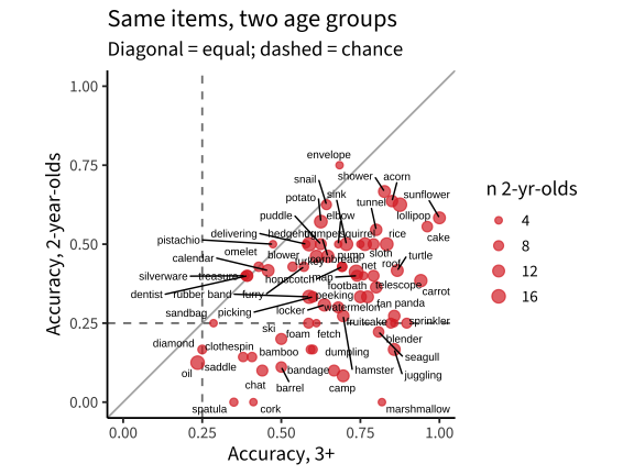
The 2-year-olds sit near chance on nearly every item regardless of how easy it is for the 3+ group — items the 3+ children get 80–90% right (panda, carrot, turtle, map) are at 0–0.35 for the 2s, and the item-level correlation between the groups is only r ≈ 0.38. If the 2-year-olds were simply weaker vocabulary learners we’d expect the same difficulty ordering, shifted down; instead the ordering is largely lost, which is what non-engagement / task-incomprehension looks like — consistent with their catch- trial failures above. A handful of items (sunflower, telescope, net, hedgehog) show some 2-year-old signal, but on 4–10 children each.
Does the 5–12 difficulty ordering hold for preschoolers?
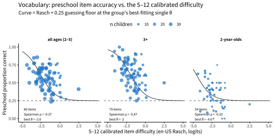
The vocabulary CAT’s item bank was calibrated on 5–12-year-olds (by_language en-US Rasch with a 0.25 guessing floor; levante_metadata_scoring v1_14, via load_item_parameters()). Every item the Boston children saw is in that calibration, so we can ask whether the 5–12 difficulty ordering survives down here — and, treating each age group as if it were a single 5–12-scale person, what θ its item accuracies imply. Curves are the model-implied P(correct) = 0.25 + 0.75·logistic(θ − b) at the group’s best-fitting θ (binomial deviance minimised over items).
Code
ip <-load_item_parameters() |>filter(task_id =="vocab", subset =="en-US") |>select(item_uid, difficulty)fit_theta <-function(k, n, b) {optimize(\(th) -sum(dbinom(k, n, 0.25+0.75*plogis(th - b), log =TRUE)), c(-8, 6))$minimum}grp_items <- vi |>mutate(grp ="all ages (2–5)") |>bind_rows(vi) |>group_by(grp, item, item_uid) |>summarise(n =n(), k =sum(correct), acc =mean(correct), .groups ="drop") |>inner_join(ip, by ="item_uid") |>filter((grp =="2-year-olds"& n >=4) | (grp !="2-year-olds"& n >=10)) |>mutate(grp =factor(grp, c("all ages (2–5)", "3+", "2-year-olds")))grp_stats <- grp_items |>group_by(grp) |>summarise(items =n(), rho =cor(acc, difficulty, method ="spearman"),theta =fit_theta(k, n, difficulty), .groups ="drop")curves <- grp_stats |>reframe(difficulty =seq(-5, 5, 0.1), .by =c(grp, theta)) |>mutate(p =0.25+0.75*plogis(theta - difficulty))ggplot(grp_items, aes(difficulty, acc)) +geom_hline(yintercept =0.25, linetype ="dashed", colour ="grey50") +geom_line(data = curves, aes(y = p), colour ="grey30") +geom_point(aes(size = n), colour ="#268bd2", alpha =0.7) +geom_text(data = grp_stats, aes(x =-4.8, y =0.06,label =glue("{items} items\nSpearman ρ = {round(rho, 2)}\nbest θ = {round(theta, 1)}")),hjust =0, size =3.2) +facet_wrap(~grp) +scale_size_area(max_size =4, name ="n children") +scale_y_continuous(limits =c(0, 1)) +labs(x ="5–12 calibrated item difficulty (en-US Rasch, logits)", y ="Preschool proportion correct",title ="Vocabulary: preschool item accuracy vs. the 5–12 calibrated difficulty",subtitle ="Curve = Rasch + 0.25 guessing floor at the group's best-fitting single θ") +theme(legend.position ="top")
Code
grp_stats |>mutate(across(c(rho, theta), ~round(.x, 2))) |> knitr::kable(caption ="Per group: items, Spearman correlation between preschool accuracy and 5–12 difficulty, and the best-fitting single θ on the 5–12 scale")
Per group: items, Spearman correlation between preschool accuracy and 5–12 difficulty, and the best-fitting single θ on the 5–12 scale
grp
items
rho
theta
all ages (2–5)
80
-0.37
-2.63
3+
79
-0.47
-2.04
2-year-olds
54
-0.33
-4.65
For the 3+ children the 5–12 ordering carries down: accuracy falls with calibrated difficulty (Spearman ρ = -0.47), and the item points sit along the Rasch curve at a single θ ≈ -2 — the 3–5 group behaves like a low-ability 5–12-scale person, which is what a downward extension of the same construct should look like. For the 2-year-olds the relation is much weaker (ρ = -0.33, fitted θ ≈ -4.6 near the guessing floor) — but with the larger sample it is no longer zero (the June tranche gave ρ ≈ −0.16): the oldest/most-engaged 2-year-olds are starting to show the same ordering. The practical implication is that the existing en-US bank plus its calibration is a plausible starting point for 3–5 — the CAT was already routing these children to the bank’s easy tail (median difficulty of items seen ≈ −1.9), and the 3+ group’s average θ ≈ -2 sits right there — but the bank thins out fast below b ≈ −3 (only 9% of the 146 en-US items; easiest −4.4). So the average 3–5-year-old is measurable, while younger/weaker children in the band (and certainly the 2-year-olds, θ ≈ -4.6) fall below where items exist. The bank needs easier items to cover this band, and 2-year-olds need something other than 4-AFC picture naming.
5. Data-quality flags to carry forward
Code
# How far down the age range does each Math subtask reach, and where is it above chance?math_h |>group_by(subtask) |>summarise(kids =n_distinct(user_id), min_age =min(age), acc_under4 =mean(acc[age <4]),acc_4plus =mean(acc[age >=4]), chance =mean(chance), .groups ="drop") |>arrange(min_age) |> knitr::kable(digits =2, caption ="Math subtasks: youngest child served, and mean accuracy below vs. above age 4 (chance shown). Under 4 nothing reliably clears chance; from 4 on the number subtasks do, while Addition stays at chance throughout")
Math subtasks: youngest child served, and mean accuracy below vs. above age 4 (chance shown). Under 4 nothing reliably clears chance; from 4 on the number subtasks do, while Addition stays at chance throughout
subtask
kids
min_age
acc_under4
acc_4plus
chance
Addition
30
2.00
0.17
0.31
0.25
Number Comparison
33
2.00
0.40
0.63
0.50
Counting AFC
21
2.17
0.29
0.60
0.33
Non-symbolic Number Identification
21
2.17
0.37
0.63
0.33
Number Identification
25
2.25
0.27
0.53
0.25
Missing Number
15
4.58
NaN
0.28
0.25
Subtraction
4
5.17
NaN
0.35
0.25
Multiplication
1
5.83
NaN
0.00
0.25
Code
# Vocabulary catch trials as an engagement gatevocab_h |>mutate(age_yr =floor(age)) |>group_by(age_yr, kind) |>summarise(runs =n(), acc =mean(acc), .groups ="drop") |>pivot_wider(names_from = kind, values_from =c(runs, acc)) |> knitr::kable(digits =2, caption ="Vocabulary: catch-trial vs test accuracy by age year")
Vocabulary: catch-trial vs test accuracy by age year
age_yr
runs_catch
runs_test
acc_catch
acc_test
2
15
17
0.50
0.38
3
11
11
0.89
0.57
4
6
11
0.83
0.60
5
3
14
1.00
0.70
Short / invalid runs concentrate at the young end (see §3.1, §3.4): the <10 test trials rule removes many 2-year-old runs — for this age band the validity floor itself needs re-thinking (a 2-year-old’s 8 valid trials may be the whole point).
2–2.5-year-olds sit at chance on the core tasks (Vocabulary 0.26, Sentence Understanding 0.31, Math at/below chance) and pass the Vocabulary catch trials only ≈ 50% (vs ≈ 90–100% from age 3) — much of the youngest data reflects partial engagement rather than measured ability. But the 2026-08 sample softens the June picture: by 2.5–3 every language/ reasoning task clears chance (Vocab 0.49, TROG 0.46, Matrix 0.51, SDS 0.74), so the practical cut for the current battery is ~2.5, not 3. Catch-trial accuracy remains a usable engagement gate.
CAT item banks are calibrated for 5–12: the top of the routing behaves sensibly (Subtraction / Multiplication reached only 5-year-olds), but the bank has no floor for this band — Addition items reach 2-year-olds yet sit at chance across the whole 2–5 range, and below age 4 no Math subtask reliably clears chance (the number subtasks do from 4 on). Running θ is not interpretable at this age.
Memory records no RT (rt_numeric all NA) — known from the main pipeline; fine for accuracy/span, no timing possible.
Same & Different staging is irregular in the raw table (first_response/second_response/… plus blank assessment_stage), and its scoring is under revision anyway (see LEVANTE.md); the SDS numbers here are proportion-correct by trial type only.
Shape Rotation trials record 2 distractors (3-AFC) in this dataset, whereas the calibrated models use a 0.5 guessing floor — check which variant ran before comparing to 5–12 data.
stop_type is entirely NA in this tranche (no early-stopping info).
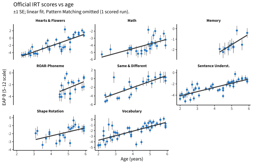
6. Official IRT scores (processed dataset)
Since the first draft of this notebook, the scoring pipeline has run: the processed dataset pilot_bostonchildrens_us_main:2fj2 (unreleased draft, pulled 2026-08-31) now carries EAP θ scores from the calibrated models for 42 of the 44 children (multigroup_dataset Rasch/2PL for the core tasks; by_language en-US for vocab/pa). These are still 5–12-calibrated models applied to 2–5-year-olds — the θs inherit every floor problem shown above — but they’re the pipeline’s official numbers.
Code
SC_REF <-"pilot_bostonchildrens_us_main:2fj2"; SC_VER <-"next-2026-08-31"sc_path <-here("data", glue("downex_boston_scores_2fj2_{SC_VER}.rds"))if (!file_exists(sc_path)) write_rds(levante::get_scores(glue("{SC_REF}:{SC_VER}")), sc_path)scores <-read_rds(sc_path) |>mutate(task = task_labels[task_id])scores |>group_by(task) |>summarise(runs =n(), scored =sum(!is.na(score)),few_valid_trials =sum(exclusion %in%"few_valid_trials"),incomplete =sum(exclusion %in%"incomplete"),no_data =sum(exclusion %in%"no_data"), .groups ="drop") |>arrange(scored / runs) |> knitr::kable(caption ="Scored vs excluded runs per task. Pattern Matching remains ~unscorable (4 of 50 runs; 26 few_valid_trials + 15 no_data): the downward-extension variant's items don't map into the calibrated bank.")
Scored vs excluded runs per task. Pattern Matching remains ~unscorable (4 of 50 runs; 26 few_valid_trials + 15 no_data): the downward-extension variant’s items don’t map into the calibrated bank.
sc_hand <- sc_ok |>inner_join(run_sum |>select(run_id, acc, n_trials), by ="run_id")sc_hand |>group_by(task) |>summarise(n =n(), r_theta_acc =cor(score, acc), r_theta_age =cor(score, age),mean_se =mean(score_se, na.rm =TRUE), .groups ="drop") |> knitr::kable(digits =2, caption ="Official θ vs our hand accuracy and age; mean posterior SE")
Official θ vs our hand accuracy and age; mean posterior SE
task
n
r_theta_acc
r_theta_age
mean_se
Hearts & Flowers
39
0.94
0.84
0.76
Math
26
0.84
0.61
0.60
Memory
13
0.90
0.75
0.53
ROAR-Phoneme
20
0.98
0.45
0.64
Same & Different
24
0.91
0.81
0.86
Sentence Underst.
48
0.93
0.82
0.44
Shape Rotation
24
0.87
0.53
0.47
Vocabulary
51
0.82
0.75
0.48
The official θs track our hand scores closely everywhere (r ≈ 0.8–1.0 with hand accuracy) — the pipeline and the hand scoring agree about ordering. The problems are the scale and the coverage: mean posterior SEs are large (≈ 0.4–0.9 vs ≈ 0.3 typical in the 5–12 data), Math θ is compressed against the bottom of its scale (all runs between −5.3 and −1.8), and the exclusion rules built for 5–12 administration (≥10 valid trials) remove most of what the youngest children produced — so the scored subset over-represents the 3+ band. Within it, Sentence Understanding and Same & Different θs show the strongest age relations (r ≈ 0.85 and 0.81).
7. Which tasks work for 2-year-olds?
The design decision this pilot feeds is which tasks to keep for the youngest band. Two views: accuracy in fine age bins, and the trial-level logistic slope of accuracy on age fit to children under 3.5 (the “lift-off” test — is there a within-band age gradient at all?).
Code
fine <- test |>filter(!(task_id =="vocab"& corpus_trial_type =="catch")) |>mutate(bin =cut(age, c(2, 2.5, 3, 3.5, 4, 5, 6), right =FALSE,labels =c("2–2.5", "2.5–3", "3–3.5", "3.5–4", "4–5", "5–6")))fine |>group_by(task, bin) |>summarise(acc =mean(correct_hand), kids =n_distinct(user_id), .groups ="drop") |>mutate(cell =glue("{sprintf('%.2f', acc)} ({kids})")) |>select(task, bin, cell) |>pivot_wider(names_from = bin, values_from = cell) |>left_join(chance_df |>mutate(chance =round(chance, 2)), by ="task") |> knitr::kable(caption ="Hand-scored accuracy (n children) by fine age bin; rightmost column = task-average chance")
Hand-scored accuracy (n children) by fine age bin; rightmost column = task-average chance
task
2–2.5
2.5–3
3–3.5
3.5–4
4–5
5–6
chance
Hearts & Flowers
0.33 (6)
0.42 (4)
0.48 (3)
0.67 (4)
0.69 (8)
0.86 (10)
0.50
Math
0.35 (4)
0.29 (4)
0.12 (2)
0.47 (3)
0.52 (9)
0.59 (11)
0.31
Memory
NA
0.00 (2)
0.00 (1)
0.28 (3)
0.51 (6)
0.57 (7)
0.00
Pattern Matching
0.25 (4)
0.51 (5)
0.45 (2)
0.50 (3)
0.53 (9)
0.48 (7)
0.25
ROAR-Phoneme
NA
NA
NA
NA
0.58 (7)
0.61 (12)
NaN
Same & Different
0.42 (5)
0.74 (3)
0.64 (2)
0.70 (4)
0.74 (6)
0.91 (5)
0.30
Sentence Underst.
0.31 (10)
0.46 (5)
0.61 (3)
0.66 (4)
0.62 (10)
0.75 (10)
0.25
Shape Rotation
NA
NA
0.55 (2)
0.55 (4)
0.54 (6)
0.74 (11)
0.33
Vocabulary
0.26 (9)
0.49 (5)
0.50 (3)
0.60 (4)
0.57 (10)
0.69 (12)
0.25
Code
liftoff <- fine |>filter(age <3.5) |>group_by(task) |>filter(n_distinct(user_id) >=4) |>group_modify(\(d, ...) { co <-summary(glm(correct_hand ~ age, binomial, d))$coefficientstibble(kids =n_distinct(d$user_id), trials =nrow(d),slope = co[2, 1], se = co[2, 2], p = co[2, 4]) }) |>ungroup() |>arrange(desc(slope))liftoff |>mutate(across(c(slope, se), ~round(.x, 2)), p =signif(p, 2)) |> knitr::kable(caption ="Lift-off under 3.5: logistic slope of trial correctness on age (logits/year), tasks with ≥4 children under 3.5")
Lift-off under 3.5: logistic slope of trial correctness on age (logits/year), tasks with ≥4 children under 3.5
task
kids
trials
slope
se
p
Vocabulary
16
891
1.44
0.20
0.0000
Sentence Underst.
17
884
1.41
0.21
0.0000
Pattern Matching
10
203
1.32
0.46
0.0037
Same & Different
10
195
1.17
0.40
0.0032
Hearts & Flowers
13
343
0.91
0.32
0.0040
Math
10
91
-0.78
0.69
0.2600
Verdict by task, for the 2s specifically:
Vocabulary — keep. Clear lift-off (+1.4 logits/yr under 3.5, p < .001, now on 16 kids / 891 trials): 2–2.5s sit at chance (0.26) but 2.5–3s are at 0.49, and 2-year-olds pass the easy catch items at 50% vs 25% chance — the format works once items are easy enough; the bank, not the task, is the problem.
Sentence Understanding — keep. Clear lift-off (+1.4 logits/yr, p < .001); 0.31 at 2–2.5 (chance .25) rising to 0.46 by 2.5–3, on the most under-3 data of any task (17 kids under 3.5).
Math — drop for 2s. Still the clearest negative: slope −0.8 (p = .26) under 3.5, at/below chance in every bin below 3.5, and the item bank has no items down there (§5).
Memory (Corsi) — drop for 2s. Complete floor: the under-3s who reached test trials got literally zero sequences correct (max span 0), and most young runs died before producing 10 valid trials.
Hearts & Flowers — borderline, leaning drop below ~3. Lift-off is real (+0.9 logits/yr, p = .004, 13 kids) but rises from below chance (0.33 at 2–2.5 on a 2-AFC — systematic perseveration/too-slow responding, not noise); it doesn’t clear chance until ~3.5.
Pattern Matching — behaviorally promising, blocked by scoring (changed verdict). With the larger sample the downward-extension variant shows clear lift-off (+1.3 logits/yr, p = .004; chance 0.25 at 2–2.5 → 0.51 at 2.5–3) — but §6 shows it is still ~unscorable against the current bank (4 of 50 runs). Calibrating the downex items is now clearly worth it.
Same & Different — promising from ~2.5 (changed verdict). Now has under-3 data (10 kids): lift-off +1.2 logits/yr (p = .003), 0.42 at 2–2.5 (chance ≈ 0.30) rising to 0.74 at 2.5–3.
Shape Rotation / ROAR-Phoneme: still almost no under-3 data; no basis to judge.
Notes & next steps
Data: pilot_bostonchildrens_us_main_raw:7e6c v5_0 (raw, per-site) + the unreleased processed draft (pulled 2026-08-31). Cached under data/ (git-ignored). Two other downward-extension raw datasets exist on Redivis — pilot_langcog_us_downex_raw:a6kb (Stanford) and partner_sparklab_us_downex_raw:4n9e — natural comparison sets once the Boston picture is clear.
In the published book (since 2026-08-17, by explicit decision); sample now N = 44.
Next: (i) decide a validity floor appropriate for 2–5; (ii) look at practice-trial performance as an engagement gate; (iii) once ≥ 2 sites of downward-extension data exist, item-level difficulty for a 2–5 bank; (iv) compare with the Stanford / Sparklab downex tranches.