Test–retest figures (corrected v1.2) — Colombia & Germany

ImportantAI-generated — not for publication

The code and prose in this chapter were written by Claude Code (an AI coding agent) under human direction. They have not been line-by-line verified by a human and must not be published or cited as-is.

WarningPreliminary & unvetted analysis

These are exploratory analyses of preliminary, in-progress LEVANTE data. Results have not been reviewed or validated and require checking by the LEVANTE Data Coordinating Center before any use.

Purpose

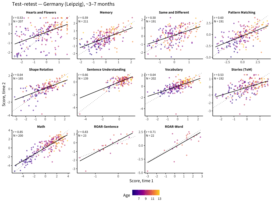
Test–retest scatter figures in the style of the core-tasks paper (Figure 4): each panel is one task, T1 score vs T2 score, points coloured by age, with the test–retest correlation r and N annotated. Two figures:

  • Colombia — Bogotá (~15-month retest interval)
  • Germany — Leipzig (~3–7-month retest interval)

On corrected (v1.2) data. Each site shows the tasks for which it has ≥ 20 two-wave children (Colombia has no ToM/Same-and-Different retest; both sites’ thin ROAR cells are dropped where < 20). Scales are per-task (free) because the tasks are on different score metrics (IRT θ; ROAR-Sentence is a z-scaled count). PNGs saved to figures/.

Code
source(here::here("common.R"))
fig_dir <- here::here("figures"); fs::dir_create(fig_dir)
sc <- read_rds(here::here("data/scores_all_sites.rds"))

cat_order <- c("Executive function","Reasoning","Spatial cognition",
               "Language","Social cognition","Math","Reading")

build_pairs <- function(ds) {
  sc |> filter(dataset == ds,
               task_id %in% c(core_task_ids, "swr", "sre", "pa"),
               !is.na(score), !is.na(age)) |>
    group_by(task_id, task_label, task_category, user_id) |>
    arrange(age) |> mutate(wave = row_number()) |> ungroup() |>
    filter(wave <= 2) |>
    group_by(task_id, task_label, task_category, user_id) |>
    filter(n_distinct(wave) == 2) |>
    summarise(t1 = score[wave == 1], t2 = score[wave == 2],
              age = age[wave == 1], .groups = "drop") |>
    group_by(task_id, task_label, task_category) |>
    filter(n() >= 20) |>
    mutate(score1 = pmin(pmax(t1, -6), 6), score2 = pmin(pmax(t2, -6), 6)) |>
    ungroup() |>
    mutate(task_category = factor(task_category, levels = cat_order),
           facet = fct_reorder(task_label, as.integer(task_category)))
}

retest_fig <- function(pairs, title) {
  labs_df <- pairs |> group_by(facet) |>
    summarise(r = cor(score1, score2, use = "complete.obs"), n = n(),
              .groups = "drop") |>
    mutate(label = sprintf("r = %.2f\nN = %d", r, n))
  ggplot(pairs, aes(x = score1, y = score2)) +
    geom_abline(slope = 1, intercept = 0, lty = 3, color = "grey55") +
    geom_point(aes(color = age), alpha = 0.55, size = 1.1) +
    geom_smooth(method = "lm", se = FALSE, color = "black", linewidth = 0.7) +
    geom_text(data = labs_df, aes(x = -Inf, y = Inf, label = label),
              hjust = -0.12, vjust = 1.15, size = 3.6, lineheight = 0.95,
              family = .levante_font) +
    facet_wrap(~facet, scales = "free") +
    scale_color_viridis_c(option = "plasma", end = 0.92, name = "Age") +
    labs(x = "Score, time 1", y = "Score, time 2", title = title) +
    theme(legend.position = "bottom",
          strip.text = element_text(face = "bold"))
}
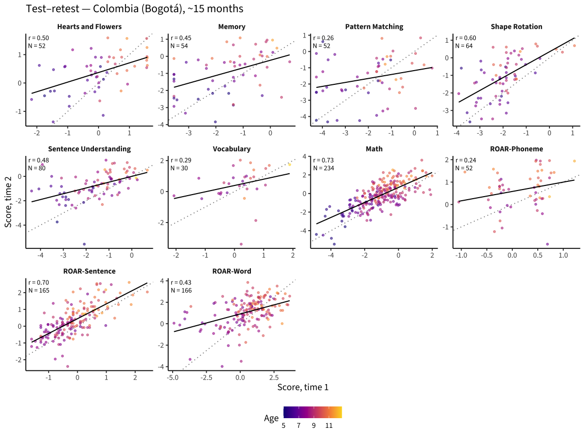
Colombia — Bogotá (~15-month retest)

Code
co <- build_pairs("pilot_uniandes_co_bogota")
p_co <- retest_fig(co, "Test–retest — Colombia (Bogotá), ~15 months")
p_co

Code
ggsave(file.path(fig_dir, "test_retest_colombia.png"), p_co,
       width = 12, height = 9, dpi = 300, bg = "white")

Germany — Leipzig (~3–7-month retest)

Code
de <- build_pairs("pilot_mpieva_de_main")
p_de <- retest_fig(de, "Test–retest — Germany (Leipzig), ~3–7 months")
p_de

Code
ggsave(file.path(fig_dir, "test_retest_germany.png"), p_de,
       width = 12, height = 9, dpi = 300, bg = "white")

Test–retest correlations

Code
bind_rows(
  build_pairs("pilot_uniandes_co_bogota") |> mutate(site = "Colombia (~15mo)"),
  build_pairs("pilot_mpieva_de_main")     |> mutate(site = "Germany (~3–7mo)")
) |>
  group_by(site, task_category, task_label) |>
  summarise(n = n(), r = cor(score1, score2, use = "complete.obs"),
            .groups = "drop") |>
  pivot_wider(names_from = site, values_from = c(n, r)) |>
  arrange(task_category, task_label) |>
  knitr::kable(digits = 2, caption = "Test–retest r by task and site")
Test–retest r by task and site
task_category task_label n_Colombia (~15mo) n_Germany (~3–7mo) r_Colombia (~15mo) r_Germany (~3–7mo)
Executive function Hearts and Flowers 52 207 0.50 0.53
Executive function Memory 54 211 0.45 0.59
Executive function Same and Different NA 191 NA 0.50
Reasoning Pattern Matching 52 191 0.26 0.60
Spatial cognition Shape Rotation 64 165 0.60 0.64
Language Sentence Understanding 80 139 0.48 0.66
Language Vocabulary 30 202 0.29 0.64
Social cognition Stories (ToM) NA 192 NA 0.53
Math Math 234 200 0.73 0.85
Reading ROAR-Phoneme 52 NA 0.24 NA
Reading ROAR-Sentence 165 23 0.70 0.83
Reading ROAR-Word 166 22 0.43 0.71

Figures saved to figures/test_retest_colombia.png and figures/test_retest_germany.png.