ROAR-Sentence (SRE) — scoring deepdive

ImportantAI-generated — not for publication

The code and prose in this chapter were written by Claude Code (an AI coding agent) under human direction. They have not been line-by-line verified by a human and must not be published or cited as-is.

WarningPreliminary & unvetted analysis

These are exploratory analyses of preliminary, in-progress LEVANTE data. Results have not been reviewed or validated and require checking by the LEVANTE Data Coordinating Center before any use.

Scope

Sentence Reading Efficiency (SRE) is a speeded literacy measure adapted from ROAR (intro-sre; Yeatman et al., 2024). Children read simple sentences one at a time and judge each true or false (2AFC), reading as many as they can in 180 seconds. ROAR’s official score is correct − incorrect within the time window — the subtraction is a guessing correction (a random guesser nets ≈ 0). LEVANTE z-scores this count within dataset so it sits on a roughly comparable scale to the IRT tasks (score_type = "guessing_adjusted_number_correct_scaled").

The scoring bug. levantemodels::score_sre() computes filter(trial_number <= 180) then (sum(correct) - sum(!correct)) / 180 — i.e. it truncates at the first 180 trials, not 180 seconds. (The /180 divisor is cosmetic: it cancels in the z-score.) This notebook asks:

  1. Timing forensics: do runs actually last 180 seconds? (Spoiler: no — there is real structure here, including double-length runs.)
  2. Corrected scoring: rate-normalize to a per-180s net-correct rate. How much do scores change? Do age / ROAR-Phoneme (PA) / ROAR-Word (SWR) correlations change, within and across sites?
  3. Efficiency scoring: discussion of correctness+RT models (drift-diffusion IRT and alternatives) plus an EZ-diffusion proof of concept on the trial data.

Data: levante_data_pilots_hackathon:fpx0:v1_1 via the new levante package, cached by tasks/_pull_sre_hackathon.R.

Code
source(here::here("common.R"))

trials_file <- here("data/hackathon_v1_1_trials_roar.rds")
if (!file.exists(trials_file))
  stop("Run tasks/_pull_sre_hackathon.R first (requires Redivis auth).")

tr_all <- read_rds(trials_file)
sc_all <- read_rds(here("data/hackathon_v1_1_scores.rds"))

dataset_pal <- set_names(
  RColorBrewer::brewer.pal(4, "Set1"),
  dataset_labels_named[c("pilot_uniandes_co_bogota", "pilot_uniandes_co_rural",
                         "pilot_mpieva_de_main", "pilot_western_ca_main")])

label_dataset <- \(df) df |>
  mutate(dataset_label = factor(dataset_labels_named[dataset],
                                levels = names(dataset_pal)))

sre <- tr_all |>
  filter(task_id == "sre") |>
  mutate(correct = as.logical(correct),
         rt_s = rt_numeric / 1000,
         corpus = sub("_[0-9]+$", "", item_uid) |> str_remove("^sre_")) |>
  label_dataset()

sre_scores_pub <- sc_all |>
  filter(task_id == "sre", !is.na(score)) |>
  label_dataset()
Code
sre |>
  group_by(dataset_label) |>
  summarise(runs = n_distinct(run_id), children = n_distinct(user_id),
            trials = n(), .groups = "drop") |>
  knitr::kable(caption = "SRE trial data by dataset (hackathon v1_1)")
SRE trial data by dataset (hackathon v1_1)
dataset_label runs children trials
Colombia — Bogotá 806 624 30832
Colombia — Caquetá/Boyacá 576 569 22474
Germany — Leipzig 151 151 7002
Canada — Ontario 91 86 7053

1. Timing forensics: is 180 seconds always 180 seconds?

Two per-run duration measures: time-on-sentences (cumulative RT — the task records per-sentence RT in ms) and wall-clock span (last minus first trial server timestamp). Neither is exactly the timer, but they bracket it: cumulative RT omits inter-trial overhead; timestamp span omits the first trial’s duration and can inflate under server lag or pauses.

Code
run_time <- sre |>
  group_by(dataset, dataset_label, run_id, user_id) |>
  summarise(n_trials = n(),
            n_corpora = n_distinct(corpus),
            cum_rt = sum(rt_s),
            span = as.numeric(difftime(max(timestamp), min(timestamp),
                                       units = "secs")),
            n_correct = sum(correct), n_incorrect = sum(!correct),
            .groups = "drop")

run_time |>
  group_by(dataset_label) |>
  summarise(across(c(cum_rt, span),
                   list(q05 = ~quantile(.x, .05), median = median,
                        q95 = ~quantile(.x, .95), max = max)),
            .groups = "drop") |>
  knitr::kable(digits = 0,
               caption = "Per-run duration (seconds): cumulative RT and wall-clock span")
Per-run duration (seconds): cumulative RT and wall-clock span
dataset_label cum_rt_q05 cum_rt_median cum_rt_q95 cum_rt_max span_q05 span_median span_q95 span_max
Colombia — Bogotá 108 160 170 174 157 180 204 369
Colombia — Caquetá/Boyacá 87 161 171 175 135 178 200 373
Germany — Leipzig 150 164 171 174 169 182 197 561
Canada — Ontario 156 166 326 342 165 176 365 404
Code
run_time |>
  ggplot(aes(x = cum_rt, fill = dataset_label)) +
  facet_wrap(vars(dataset_label), scales = "free_y") +
  geom_histogram(binwidth = 10, boundary = 0, show.legend = FALSE) +
  geom_vline(xintercept = 180, lty = 2) +
  scale_fill_manual(values = dataset_pal) +
  labs(x = "Cumulative RT per run (s)", y = "Runs",
       title = "Most runs sum to just under 180 s of reading time",
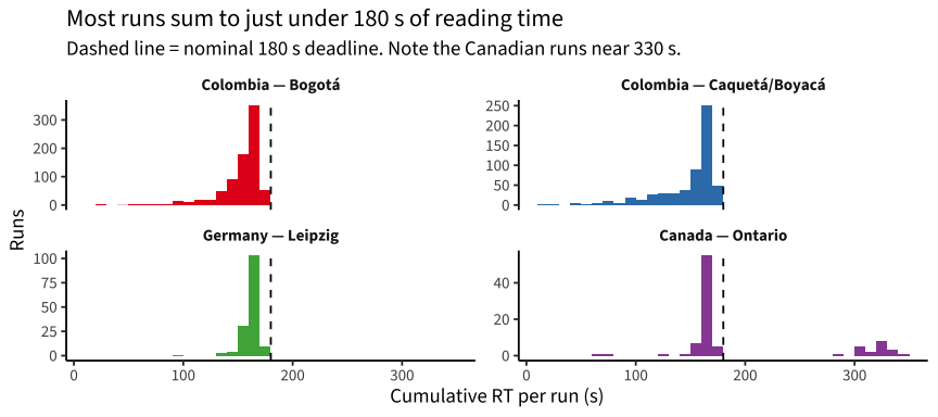
       subtitle = "Dashed line = nominal 180 s deadline. Note the Canadian runs near 330 s.")

Three regularities:

  • The 180 s deadline is real but not exact. Median time-on-sentences is ~160–165 s (the remainder is inter-trial overhead: wall-clock span medians ~180 s). So the timer fires on schedule for most runs.
  • A left tail of short runs exists everywhere — Colombia especially (rural 5th percentile ≈ 87 s of reading time). Under the current rule these short runs are scored as if the child had the full window.
  • Canada (Western) has genuinely double-length runs.

Block structure: some Canadian runs contain two 180-s blocks

The item bank prefix identifies sentence corpora. Colombia interleaves three corpora (spanish_lab, spanish_ai, spanish_ai-human) within one timed block; Germany uses one corpus (uzh). But 20 Canadian runs contain two sequential blocks (lab sentences, then ai sentences), each with its own ~180-s window — roughly 360 s of testing scored as if it were one window.

Code
run_blocks <- sre |>
  group_by(dataset_label, run_id, corpus) |>
  summarise(block_rt = sum(rt_s), n = n(), .groups = "drop_last") |>
  summarise(blocks = paste(sort(corpus), collapse = " + "),
            two_windows = sum(block_rt > 120) >= 2,
            .groups = "drop")

run_blocks |>
  count(dataset_label, blocks, two_windows) |>
  arrange(dataset_label, desc(n)) |>
  knitr::kable(caption = "Corpus composition of runs. two_windows = ≥2 corpora each with >120 s of reading time (sequential blocks, not interleaving)")
Corpus composition of runs. two_windows = ≥2 corpora each with >120 s of reading time (sequential blocks, not interleaving)
dataset_label blocks two_windows n
Colombia — Bogotá spanish_ai + spanish_ai-human + spanish_lab FALSE 785
Colombia — Bogotá spanish_ai + spanish_lab FALSE 20
Colombia — Bogotá spanish_ai + spanish_ai-human FALSE 1
Colombia — Caquetá/Boyacá spanish_ai + spanish_ai-human + spanish_lab FALSE 563
Colombia — Caquetá/Boyacá spanish_ai + spanish_lab FALSE 13
Germany — Leipzig uzh FALSE 151
Canada — Ontario aiV1P1 FALSE 27
Canada — Ontario lab FALSE 25
Canada — Ontario ai + lab TRUE 20
Canada — Ontario aiV1P2 FALSE 19
Code
run_time |>
  ggplot(aes(x = n_trials, fill = dataset_label)) +
  facet_wrap(vars(dataset_label), scales = "free_y") +
  geom_histogram(binwidth = 10, boundary = 0, show.legend = FALSE) +
  geom_vline(xintercept = 180, lty = 2) +
  scale_fill_manual(values = dataset_pal) +
  labs(x = "Trials per run", y = "Runs",
       title = "Only Canada ever reaches the 180-trial truncation point",
       subtitle = "Dashed line = the current rule's truncation at 180 trials")

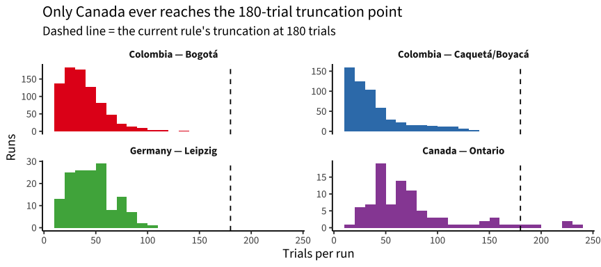
Side-quest verdict: the first-180-trials filter is a no-op for Germany and Colombia (no run exceeds 180 trials — max 140). It bites only in Canada (5 runs exceed 180 trials, max 238), and there it truncates arbitrarily across the two-block structure. Meanwhile the actual problem is the reverse: effective testing time varies from ~1 to ~4 minutes across runs, and a raw count treats them all as equal.

2. Corrected scoring: rate normalization

The corrected score is a rate: net correct per 180 s of reading time,

\[\text{score} = \frac{C - I}{\text{cumulative RT (s)}} \times 180,\]

then z-scored within dataset (preserving the pipeline’s scaling convention). We use time-on-sentences rather than wall-clock span as the denominator because it is robust to server-timestamp lag and pauses; the two agree closely (sensitivity check below). Runs with under 30 s of reading time are excluded from rate scoring (extrapolation too aggressive).

First, verify we can reproduce the published (buggy) scores exactly:

Code
old_score <- sre |>
  group_by(dataset, run_id) |>
  filter(trial_number <= 180) |>
  summarise(net = sum(correct) - sum(!correct), .groups = "drop") |>
  group_by(dataset) |>
  mutate(score_old = scale(net)[, 1]) |>
  ungroup()

old_score |>
  inner_join(sre_scores_pub, by = c("dataset", "run_id")) |>
  group_by(dataset_label) |>
  summarise(n = n(), r_with_published = cor(score_old, score), .groups = "drop") |>
  knitr::kable(digits = 3,
               caption = "Local reimplementation of the current rule vs published scores (r ≈ 1; residual differences come from a few scored runs with no rows in the trials table, which shift the z-scale slightly)")
Local reimplementation of the current rule vs published scores (r ≈ 1; residual differences come from a few scored runs with no rows in the trials table, which shift the z-scale slightly)
dataset_label n r_with_published
Colombia — Bogotá 806 1
Colombia — Caquetá/Boyacá 576 1
Germany — Leipzig 151 1
Canada — Ontario 91 1
Code
min_time <- 30

new_score <- run_time |>
  filter(cum_rt >= min_time) |>
  mutate(rate = (n_correct - n_incorrect) / cum_rt * 180) |>
  group_by(dataset) |>
  mutate(score_new = scale(rate)[, 1]) |>
  ungroup()

scores_cmp <- new_score |>
  inner_join(old_score |> select(dataset, run_id, net, score_old),
             by = c("dataset", "run_id")) |>
  left_join(sre_scores_pub |> select(dataset, run_id, age),
            by = c("dataset", "run_id"))

Excluded by the 30-s floor: 4 runs.

A) How much do scores change?

Code
cors <- scores_cmp |>
  group_by(dataset_label) |>
  summarise(n = n(), r = cor(score_old, score_new),
            r_spearman = cor(score_old, score_new, method = "spearman"),
            mean_abs_change = mean(abs(score_new - score_old)),
            max_abs_change = max(abs(score_new - score_old)),
            .groups = "drop")

knitr::kable(cors, digits = 2,
             caption = "Current (first-180-trials) vs corrected (rate per 180 s) z-scores")
Current (first-180-trials) vs corrected (rate per 180 s) z-scores
dataset_label n r r_spearman mean_abs_change max_abs_change
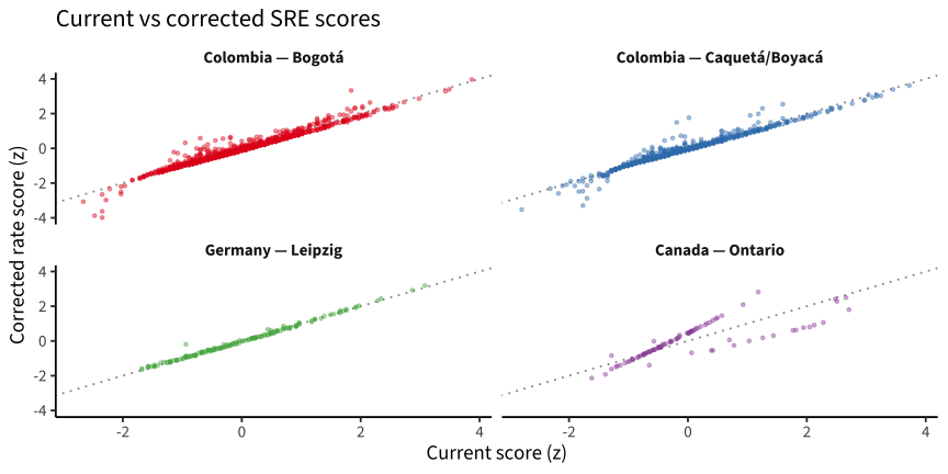
Colombia — Bogotá 804 0.98 0.98 0.13 1.64
Colombia — Caquetá/Boyacá 574 0.97 0.98 0.13 1.75
Germany — Leipzig 151 1.00 0.99 0.05 0.75
Canada — Ontario 91 0.82 0.90 0.45 1.64
Code
scores_cmp |>
  ggplot(aes(x = score_old, y = score_new, color = dataset_label)) +
  facet_wrap(vars(dataset_label)) +
  geom_abline(lty = 3, color = "grey60") +
  geom_point(alpha = 0.4, size = 0.8, show.legend = FALSE) +
  scale_color_manual(values = dataset_pal) +
  labs(x = "Current score (z)", y = "Corrected rate score (z)",
       title = "Current vs corrected SRE scores")

Code
scores_cmp |>
  mutate(change = score_new - score_old) |>
  slice_max(abs(change), n = 10) |>
  select(dataset_label, run_id, n_trials, cum_rt, n_correct, n_incorrect,
         score_old, score_new, change) |>
  knitr::kable(digits = 2, caption = "Largest score changes under rate normalization")
Largest score changes under rate normalization
dataset_label run_id n_trials cum_rt n_correct n_incorrect score_old score_new change
Colombia — Caquetá/Boyacá mKuTNWcxCzrGcj7fw3Jp 109 62.12 63 46 0.02 1.76 1.75
Colombia — Caquetá/Boyacá NBTsafmte9hxaoF3Gcds 106 56.45 60 46 -0.19 1.49 1.68
Canada — Ontario UmSVmrEZ5QpZG1zCTrIu 116 147.31 113 3 1.18 2.82 1.64
Colombia — Bogotá boJOZu6tFNABDarWSv0l 93 45.52 41 52 -2.35 -3.98 -1.64
Colombia — Caquetá/Boyacá YD6WgIH5nHRSj6WoQHdW 105 43.76 48 57 -1.77 -3.29 -1.53
Colombia — Bogotá 5QWWlNQzCeAnI0woscJG 63 108.16 59 4 1.84 3.33 1.49
Colombia — Bogotá MopLVdaKTIVBZWrQbNri 107 56.39 47 60 -2.47 -3.88 -1.40
Colombia — Bogotá RFtdYXOjnaMWdVeXNsUN 111 66.05 63 48 -0.70 0.59 1.29
Colombia — Bogotá YoQMu5bPmjFQ0XB8mTUP 89 53.66 39 50 -2.35 -3.63 -1.28
Colombia — Bogotá x5g3BStxxDNOtzRGOXE6 99 55.16 55 44 -0.95 0.32 1.27
Code
scores_cmp |>
  mutate(change = score_new - score_old) |>
  ggplot(aes(x = cum_rt, y = change, color = dataset_label)) +
  geom_hline(yintercept = 0, lty = 3) +
  geom_vline(xintercept = 180, lty = 2, color = "grey60") +
  geom_point(alpha = 0.5, size = 0.9) +
  scale_color_manual(values = dataset_pal, name = NULL) +
  labs(x = "Cumulative RT per run (s)", y = "Corrected − current (z)",
       title = "Who moves: short runs move up, double-length runs move down") +
  theme(legend.position = "bottom")

B) Validity correlations, current vs corrected

Within each dataset: correlations of SRE with age, ROAR-Phoneme (θ), and ROAR-Word (θ). Cross-run joins take each child’s first run per task.

Code
first_run <- \(df) df |>
  group_by(dataset, user_id) |>
  arrange(time_started) |>
  slice(1) |>
  ungroup()

pa_swr <- sc_all |>
  filter(task_id %in% c("pa", "swr"), !is.na(score)) |>
  first_run() |>
  select(dataset, user_id, task_id, other = score) |>
  pivot_wider(names_from = task_id, values_from = other)

sre_first <- sre_scores_pub |>
  first_run() |>
  select(dataset, dataset_label, user_id, run_id, age) |>
  inner_join(scores_cmp |> select(dataset, run_id, score_old, score_new),
             by = c("dataset", "run_id")) |>
  left_join(pa_swr, by = c("dataset", "user_id"))

validity <- sre_first |>
  pivot_longer(c(age, pa, swr), names_to = "criterion", values_to = "crit") |>
  filter(!is.na(crit)) |>
  group_by(dataset_label, criterion) |>
  filter(n() >= 20) |>
  summarise(n = n(),
            r_current = cor(score_old, crit),
            r_corrected = cor(score_new, crit), .groups = "drop") |>
  mutate(delta = r_corrected - r_current)

knitr::kable(validity, digits = 2,
             caption = "SRE validity correlations within dataset, current vs corrected scoring")
SRE validity correlations within dataset, current vs corrected scoring
dataset_label criterion n r_current r_corrected delta
Colombia — Bogotá age 533 0.60 0.60 0.00
Colombia — Bogotá pa 365 0.44 0.45 0.00
Colombia — Bogotá swr 198 0.55 0.57 0.02
Colombia — Caquetá/Boyacá age 567 0.44 0.42 -0.03
Colombia — Caquetá/Boyacá pa 557 0.59 0.57 -0.02
Germany — Leipzig age 151 0.54 0.54 0.01
Germany — Leipzig swr 150 0.59 0.58 -0.01
Canada — Ontario age 86 0.32 0.39 0.08
Canada — Ontario pa 69 0.45 0.42 -0.03
Code
pooled <- sre_first |>
  pivot_longer(c(age, pa, swr), names_to = "criterion", values_to = "crit") |>
  filter(!is.na(crit)) |>
  group_by(criterion) |>
  summarise(n = n(),
            r_current = cor(score_old, crit),
            r_corrected = cor(score_new, crit), .groups = "drop") |>
  mutate(delta = r_corrected - r_current)

knitr::kable(pooled, digits = 2,
             caption = "Pooled across datasets (all scores z-scaled within dataset; PA/SWR θ are by-language, so pooled r mixes calibrations — interpret within-site values first)")
Pooled across datasets (all scores z-scaled within dataset; PA/SWR θ are by-language, so pooled r mixes calibrations — interpret within-site values first)
criterion n r_current r_corrected delta
age 1337 0.50 0.49 -0.01
pa 991 0.44 0.45 0.00
swr 370 0.54 0.53 -0.01

Longitudinal stability (Bogotá, ~16-month gap)

Bogotá has ~180 children with SRE at two waves. Rank-order stability across 16 months is a demanding criterion: a better score should preserve more true-score variance.

Code
stab <- sre_scores_pub |>
  filter(dataset == "pilot_uniandes_co_bogota") |>
  inner_join(scores_cmp |> select(dataset, run_id, score_old, score_new),
             by = c("dataset", "run_id")) |>
  group_by(user_id) |>
  filter(n() >= 2) |>
  arrange(time_started) |>
  summarise(gap_days = as.numeric(difftime(time_started[2], time_started[1],
                                           units = "days")),
            across(c(score_old, score_new), list(t1 = ~.x[1], t2 = ~.x[2])),
            .groups = "drop") |>
  filter(gap_days > 300)

tibble(
  n_pairs = nrow(stab),
  median_gap_months = round(median(stab$gap_days) / 30.4, 1),
  stability_current = cor(stab$score_old_t1, stab$score_old_t2),
  stability_corrected = cor(stab$score_new_t1, stab$score_new_t2)
) |>
  knitr::kable(digits = 2, caption = "16-month rank-order stability, current vs corrected")
16-month rank-order stability, current vs corrected
n_pairs median_gap_months stability_current stability_corrected
181 16.1 0.7 0.72

Sensitivity: denominator choice

Code
sens <- run_time |>
  filter(cum_rt >= min_time, span >= min_time) |>
  mutate(rate_rt = (n_correct - n_incorrect) / cum_rt * 180,
         rate_span = (n_correct - n_incorrect) / span * 180) |>
  group_by(dataset_label) |>
  summarise(n = n(), r_rt_vs_span = cor(rate_rt, rate_span), .groups = "drop")

knitr::kable(sens, digits = 3,
             caption = "Rate via cumulative RT vs via wall-clock span")
Rate via cumulative RT vs via wall-clock span
dataset_label n r_rt_vs_span
Colombia — Bogotá 804 0.973
Colombia — Caquetá/Boyacá 573 0.975
Germany — Leipzig 151 0.994
Canada — Ontario 91 0.994

3. Fast guessing: the bridge to model-based scoring

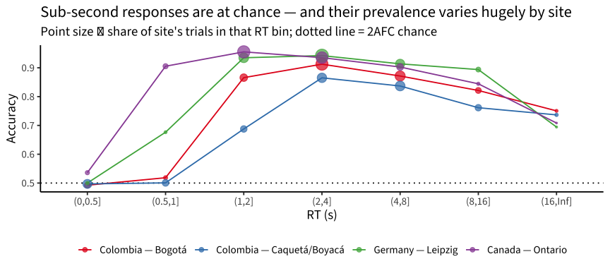
The C − I correction neutralizes guessing in expectation (a guesser nets ≈ 0), but guessing still costs signal: guessed trials burn testing time and add noise. And guessing is far from uniform across sites:

Code
sre |>
  mutate(rt_bin = cut(rt_s, c(0, .5, 1, 2, 4, 8, 16, Inf))) |>
  group_by(dataset_label, rt_bin) |>
  summarise(accuracy = mean(correct), pct = n(), .groups = "drop_last") |>
  mutate(pct = pct / sum(pct)) |>
  ungroup() |>
  ggplot(aes(x = rt_bin, y = accuracy, color = dataset_label,
             group = dataset_label)) +
  geom_hline(yintercept = 0.5, lty = 3) +
  geom_line() +
  geom_point(aes(size = pct), alpha = 0.7) +
  scale_color_manual(values = dataset_pal, name = NULL) +
  scale_size_area(max_size = 6, guide = "none") +
  labs(x = "RT (s)", y = "Accuracy",
       title = "Sub-second responses are at chance — and their prevalence varies hugely by site",
       subtitle = "Point size ∝ share of site's trials in that RT bin; dotted line = 2AFC chance") +
  theme(legend.position = "bottom")

Code
sre |>
  group_by(dataset_label) |>
  summarise(pct_rt_under_1s = mean(rt_s < 1),
            acc_under_1s = mean(correct[rt_s < 1]),
            acc_over_1s = mean(correct[rt_s >= 1]), .groups = "drop") |>
  knitr::kable(digits = 2, caption = "Fast-guessing prevalence by dataset")
Fast-guessing prevalence by dataset
dataset_label pct_rt_under_1s acc_under_1s acc_over_1s
Colombia — Bogotá 0.11 0.50 0.88
Colombia — Caquetá/Boyacá 0.31 0.50 0.81
Germany — Leipzig 0.03 0.57 0.93
Canada — Ontario 0.09 0.76 0.94

This is a strong argument for scoring models that use the joint (correct, RT) signal per trial, rather than counts alone.

4. Toward an efficiency score from correctness + RT

The modeling landscape

SRE’s design — self-paced 2AFC trials under a global deadline, with per-trial RT and accuracy — admits several principled treatments:

  1. Rate normalization (implemented above). Minimal fix: net correct per unit time. Already a speed–accuracy composite; requires no model. Its weakness: it treats a slow-and-accurate child and a fast-and-sloppy child with equal net rates as identical, and fast guessing adds noise it can only average over.

  2. Count models (Rasch Poisson counts / offset-Poisson GLMM). The classical psychometrics of speed tests (Rasch, 1960): model the count of correct responses with a log link and offset(log(time)), giving each child a latent log-rate; corpus/site enter as fixed effects, children as random effects. This is rate normalization done as a measurement model — it handles varying time windows natively and yields standard errors. It still ignores per-trial RT structure.

  3. Diffusion IRT (van der Maas et al., 2011; Molenaar et al., 2015; diffIRT, or GLMM approximations). Each trial’s (choice, RT) is a Wiener first-passage process; person drift rate \(v\) is reading efficiency, boundary separation \(a\) is caution, \(T_{er}\) is encoding/motor time. Items get drift/boundary loadings. This cleanly separates ability from speed–accuracy tradeoff and soaks up fast guesses (they are low-drift/low-boundary behavior, not ability). Cost: heavy estimation; item-level calibration needs coverage (fine in Colombia at ~60–80 runs per item; thin in Canada at ~9).

  4. Hierarchical speed–accuracy models (van der Linden, 2007). Separate IRT model for accuracy and lognormal model for RT, with correlated person ability θ and speed τ. Less mechanistic than the diffusion model; scales well; efficiency is a composite of θ and τ.

  5. Signed residual time scoring (Maris & van der Maas, 2012). Score \((2x - 1)(d - t)\) per item — correct-and-fast is best, wrong-and-fast is worst. Elegant and provably optimal under a specific IRT model, but it assumes a per-item deadline \(d\); SRE has only a global deadline, so \(d\) would be an arbitrary pseudo-deadline. Not a natural fit.

Zero-filled IRT (ROAR-team suggestion)

The ROAR team has begun exploring a simple item-based approach: fill the response matrix with zeros for unreached items, then fit a standard IRT model. Speed enters the score through the block of zeros — a fast accurate reader clears more of the bank. We fit one dense Rasch model per item bank (Spanish: Bogotá + rural jointly, 1,382 runs × 376 items; German: 151 × 200; English: 91 × 530 after dropping 18 never-reached items; _fit_sre_zerofill_irt.R).

Code
zf <- read_rds(here("data/sre_zerofill_scores.rds")) |>
  group_by(dataset) |>
  mutate(zf_z = scale(theta_zerofill)[, 1]) |>
  ungroup()

zf_first <- sre_first |>
  inner_join(zf |> select(dataset, run_id, zf_z), by = c("dataset", "run_id"))

zf_first |>
  pivot_longer(c(age, pa, swr), names_to = "criterion", values_to = "crit") |>
  filter(!is.na(crit)) |>
  group_by(dataset_label, criterion) |>
  filter(n() >= 20) |>
  summarise(n = n(),
            r_rate = cor(score_new, crit),
            r_zerofill = cor(zf_z, crit), .groups = "drop") |>
  knitr::kable(digits = 2,
               caption = "Zero-filled Rasch vs corrected rate score: validity")
Zero-filled Rasch vs corrected rate score: validity
dataset_label criterion n r_rate r_zerofill
Colombia — Bogotá age 533 0.60 0.49
Colombia — Bogotá pa 365 0.45 0.27
Colombia — Bogotá swr 198 0.57 0.51
Colombia — Caquetá/Boyacá age 567 0.42 0.19
Colombia — Caquetá/Boyacá pa 557 0.57 0.27
Germany — Leipzig age 151 0.54 0.54
Germany — Leipzig swr 150 0.58 0.56
Canada — Ontario age 86 0.39 0.31
Canada — Ontario pa 69 0.42 0.40
Code
zf_stab <- sre_scores_pub |>
  filter(dataset == "pilot_uniandes_co_bogota") |>
  inner_join(zf |> select(dataset, run_id, zf_z), by = c("dataset", "run_id")) |>
  inner_join(scores_cmp |> select(dataset, run_id, score_new),
             by = c("dataset", "run_id")) |>
  group_by(user_id) |>
  filter(n() >= 2) |>
  arrange(time_started) |>
  summarise(gap = as.numeric(difftime(time_started[2], time_started[1],
                                      units = "days")),
            across(c(zf_z, score_new), list(t1 = ~.x[1], t2 = ~.x[2])),
            .groups = "drop") |>
  filter(gap > 300)

tibble(n_pairs = nrow(zf_stab),
       rate = cor(zf_stab$score_new_t1, zf_stab$score_new_t2),
       zerofill = cor(zf_stab$zf_z_t1, zf_stab$zf_z_t2)) |>
  knitr::kable(digits = 2,
               caption = "Bogotá 16-month stability: zero-filled Rasch vs corrected rate")
Bogotá 16-month stability: zero-filled Rasch vs corrected rate
n_pairs rate zerofill
181 0.72 0.72
Code
guess_share <- sre |>
  group_by(dataset, run_id) |>
  summarise(pct_fast = mean(rt_s < 1), .groups = "drop")

zf_first |>
  inner_join(guess_share, by = c("dataset", "run_id")) |>
  group_by(dataset_label) |>
  summarise(n = n(),
            r_rate_fastguess = cor(score_new, pct_fast),
            r_zerofill_fastguess = cor(zf_z, pct_fast), .groups = "drop") |>
  knitr::kable(digits = 2,
               caption = "Correlation of each score with a run's fast-guess share (RT < 1 s). Positive = the score REWARDS guessing")
Correlation of each score with a run’s fast-guess share (RT < 1 s). Positive = the score REWARDS guessing
dataset_label n r_rate_fastguess r_zerofill_fastguess
Colombia — Bogotá 622 -0.36 0.19
Colombia — Caquetá/Boyacá 567 -0.42 0.46
Germany — Leipzig 151 -0.10 0.10
Canada — Ontario 86 0.04 0.24

Where behavior is clean, zero-fill is essentially the rate score by another route: r = .94 with the corrected rate in Germany, near-identical validity there, and Bogotá 16-month stability a statistical tie (.72 vs .72). But it has no guessing correction: a fast guesser converts wasted trials into lucky 1s among the zeros, so the score correlates positively with a run’s fast-guess share (+.46 in rural Colombia) where the rate score correlates negatively (−.42), and validity collapses exactly there (rural PA r = .27 vs .57; rural age .19 vs .42).

The obvious repair — a fixed 2AFC guessing floor (Rasch with g = .5, as in the LEVANTE multiple-choice models) — backfires: unreached items are structural zeros, and whole-bank accuracy (~10% for a typical run) sits far below any g = .5 floor, so the model cannot represent the data (EM fails to converge; validity collapses everywhere, e.g. rural age r = .08). The floor is right for “attempted and guessed,” wrong for “never reached.” A repaired variant would need a different treatment of the two zero types — at which point the model is no longer the simple suggestion, and the rate score already does the job.

Proof of concept: EZ-diffusion per run

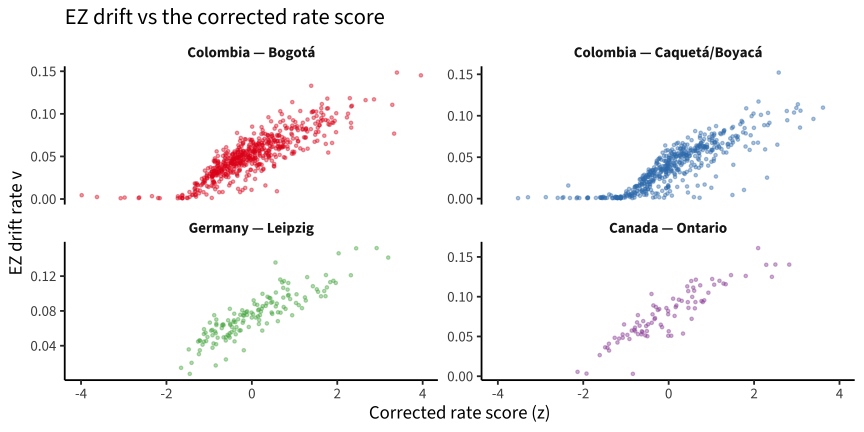
The EZ-diffusion model (Wagenmakers, van der Maas, & Grasman, 2007) inverts the simple diffusion model from three per-person summary statistics (accuracy, mean and variance of correct RTs) — no item structure, no iterative fitting. It is the cheapest possible test of whether diffusion-style decomposition adds validity beyond the rate score.

Code
ez_diffusion <- function(pc, vrt, mrt, s = 0.1) {
  s2 <- s^2
  L <- qlogis(pc)
  x <- L * (L * pc^2 - L * pc + pc - 0.5) / vrt
  v <- sign(pc - 0.5) * s * x^(1 / 4)
  a <- s2 * L / v
  y <- -v * a / s2
  mdt <- (a / (2 * v)) * (1 - exp(y)) / (1 + exp(y))
  tibble(drift = v, boundary = a, ter = mrt - mdt)
}

ez_run <- sre |>
  filter(rt_s >= 0.25, rt_s <= 30) |>
  group_by(dataset, dataset_label, run_id, user_id) |>
  filter(n() >= 15, sum(correct) >= 10) |>
  summarise(n = n(), pc_raw = mean(correct),
            mrt = mean(rt_s[correct]), vrt = var(rt_s[correct]),
            .groups = "drop") |>
  # edge-correct accuracy away from 0.5 and 1
  mutate(pc = pmin(pmax(pc_raw, 0.5 + 1 / (2 * n)), 1 - 1 / (2 * n)))

ez_run <- bind_cols(ez_run, ez_diffusion(ez_run$pc, ez_run$vrt, ez_run$mrt))

ez_run |>
  group_by(dataset_label) |>
  summarise(n_runs = n(), across(c(drift, boundary, ter), median),
            .groups = "drop") |>
  knitr::kable(digits = 2, caption = "Median EZ-diffusion parameters by dataset")
Median EZ-diffusion parameters by dataset
dataset_label n_runs drift boundary ter
Colombia — Bogotá 752 0.05 0.40 1.36
Colombia — Caquetá/Boyacá 505 0.04 0.41 1.55
Germany — Leipzig 143 0.08 0.36 1.41
Canada — Ontario 91 0.08 0.36 0.74
Code
ez_first <- sre_first |>
  inner_join(ez_run |> select(dataset, run_id, drift, boundary, ter),
             by = c("dataset", "run_id"))

ez_validity <- ez_first |>
  pivot_longer(c(age, pa, swr), names_to = "criterion", values_to = "crit") |>
  filter(!is.na(crit)) |>
  group_by(dataset_label, criterion) |>
  filter(n() >= 20) |>
  summarise(n = n(),
            r_corrected_rate = cor(score_new, crit),
            r_drift = cor(drift, crit),
            r_boundary = cor(boundary, crit), .groups = "drop")

knitr::kable(ez_validity, digits = 2,
             caption = "EZ drift vs corrected rate score: validity correlations")
EZ drift vs corrected rate score: validity correlations
dataset_label criterion n r_corrected_rate r_drift r_boundary
Colombia — Bogotá age 490 0.59 0.48 -0.12
Colombia — Bogotá pa 319 0.42 0.43 0.06
Colombia — Bogotá swr 196 0.57 0.46 -0.21
Colombia — Caquetá/Boyacá age 499 0.39 0.40 -0.04
Colombia — Caquetá/Boyacá pa 491 0.56 0.52 -0.09
Germany — Leipzig age 143 0.52 0.37 -0.24
Germany — Leipzig swr 142 0.53 0.56 -0.18
Canada — Ontario age 86 0.39 0.34 -0.29
Canada — Ontario pa 69 0.42 0.41 -0.09
Code
ez_stab <- sre_scores_pub |>
  filter(dataset == "pilot_uniandes_co_bogota") |>
  inner_join(ez_run |> select(dataset, run_id, drift),
             by = c("dataset", "run_id")) |>
  inner_join(scores_cmp |> select(dataset, run_id, score_new),
             by = c("dataset", "run_id")) |>
  group_by(user_id) |>
  filter(n() >= 2) |>
  arrange(time_started) |>
  summarise(gap = as.numeric(difftime(time_started[2], time_started[1],
                                      units = "days")),
            drift_t1 = drift[1], drift_t2 = drift[2],
            rate_t1 = score_new[1], rate_t2 = score_new[2], .groups = "drop") |>
  filter(gap > 300)

tibble(n_pairs = nrow(ez_stab),
       stability_rate = cor(ez_stab$rate_t1, ez_stab$rate_t2),
       stability_drift = cor(ez_stab$drift_t1, ez_stab$drift_t2)) |>
  knitr::kable(digits = 2,
               caption = "Bogotá 16-month stability: corrected rate vs EZ drift")
Bogotá 16-month stability: corrected rate vs EZ drift
n_pairs stability_rate stability_drift
168 0.7 0.44
Code
ez_first |>
  ggplot(aes(x = score_new, y = drift, color = dataset_label)) +
  facet_wrap(vars(dataset_label), scales = "free_y") +
  geom_point(alpha = 0.4, size = 0.8, show.legend = FALSE) +
  scale_color_manual(values = dataset_pal) +
  labs(x = "Corrected rate score (z)", y = "EZ drift rate v",
       title = "EZ drift vs the corrected rate score")

Hierarchical speed–accuracy model (van der Linden 2007 style)

The next rung up from EZ: model accuracy and RT jointly but separately, with crossed run × item random effects (fit by _fit_sre_hierarchical_sa.R):

  • accuracy: correct ~ 0 + dataset + (1|run_id) + (1|item_uid) (logit GLMM) → run-level ability θ, with item easiness absorbed by item effects (the “IRT part” that EZ lacks);
  • speed: log(rt) ~ 0 + dataset + (1|run_id) + (1|item_uid) (lognormal LMM) → run-level speed τ (sign-flipped RT effect), with item time-intensities absorbed.

An efficiency composite is z(θ) + z(τ), standardized within dataset.

Code
sa_file <- here("data/sre_sa_estimates.rds")
sa <- read_rds(sa_file)

sa_run <- sa$run |>
  group_by(dataset) |>
  mutate(theta_z = scale(theta)[, 1], tau_z = scale(tau)[, 1],
         eff = scale(theta_z + tau_z)[, 1]) |>
  ungroup()

sa_run |>
  label_dataset() |>
  group_by(dataset_label) |>
  summarise(n_runs = n(), r_theta_tau = cor(theta, tau), .groups = "drop") |>
  knitr::kable(digits = 2,
               caption = "Ability–speed correlation by dataset: near zero in DE/Canada, strongly NEGATIVE in rural Colombia — 'fast' there mostly means guessing")
Ability–speed correlation by dataset: near zero in DE/Canada, strongly NEGATIVE in rural Colombia — ‘fast’ there mostly means guessing
dataset_label n_runs r_theta_tau
Colombia — Bogotá 806 -0.23
Colombia — Caquetá/Boyacá 576 -0.52
Germany — Leipzig 151 0.01
Canada — Ontario 91 0.04
Code
sa_first <- sre_first |>
  inner_join(sa_run |> select(dataset, run_id, theta_z, tau_z, eff),
             by = c("dataset", "run_id"))

sa_first |>
  pivot_longer(c(age, pa, swr), names_to = "criterion", values_to = "crit") |>
  filter(!is.na(crit)) |>
  group_by(dataset_label, criterion) |>
  filter(n() >= 20) |>
  summarise(n = n(),
            r_rate = cor(score_new, crit),
            r_theta = cor(theta_z, crit),
            r_tau = cor(tau_z, crit),
            r_composite = cor(eff, crit), .groups = "drop") |>
  knitr::kable(digits = 2,
               caption = "Hierarchical SA model vs corrected rate score: validity")
Hierarchical SA model vs corrected rate score: validity
dataset_label criterion n r_rate r_theta r_tau r_composite
Colombia — Bogotá age 533 0.60 0.41 0.23 0.54
Colombia — Bogotá pa 365 0.45 0.47 0.01 0.40
Colombia — Bogotá swr 198 0.57 0.33 0.32 0.55
Colombia — Caquetá/Boyacá age 567 0.42 0.43 -0.15 0.28
Colombia — Caquetá/Boyacá pa 557 0.57 0.49 -0.09 0.42
Germany — Leipzig age 151 0.54 0.25 0.49 0.53
Germany — Leipzig swr 150 0.58 0.48 0.44 0.65
Canada — Ontario age 86 0.39 0.22 0.31 0.38
Canada — Ontario pa 69 0.42 0.40 0.20 0.41
Code
sa_stab <- sre_scores_pub |>
  filter(dataset == "pilot_uniandes_co_bogota") |>
  inner_join(sa_run |> select(dataset, run_id, theta_z, tau_z, eff),
             by = c("dataset", "run_id")) |>
  inner_join(scores_cmp |> select(dataset, run_id, score_new),
             by = c("dataset", "run_id")) |>
  group_by(user_id) |>
  filter(n() >= 2) |>
  arrange(time_started) |>
  summarise(gap = as.numeric(difftime(time_started[2], time_started[1],
                                      units = "days")),
            across(c(theta_z, tau_z, eff, score_new),
                   list(t1 = ~.x[1], t2 = ~.x[2])), .groups = "drop") |>
  filter(gap > 300)

tibble(n_pairs = nrow(sa_stab),
       rate = cor(sa_stab$score_new_t1, sa_stab$score_new_t2),
       theta = cor(sa_stab$theta_z_t1, sa_stab$theta_z_t2),
       tau = cor(sa_stab$tau_z_t1, sa_stab$tau_z_t2),
       composite = cor(sa_stab$eff_t1, sa_stab$eff_t2)) |>
  knitr::kable(digits = 2,
               caption = "Bogotá 16-month stability: SA-model scores vs corrected rate")
Bogotá 16-month stability: SA-model scores vs corrected rate
n_pairs rate theta tau composite
181 0.72 0.31 0.46 0.68

The decomposition is diagnostic gold but scoring lead. The ability–speed correlation flips sign across sites (≈ 0 in DE/Canada, −.23 Bogotá, −.52 rural CO): where fast guessing is common, the “speed” dimension is contaminated by disengagement, so neither τ nor any fixed θ+τ composite travels across sites. The composite matches the rate score where behavior is clean (r ≈ .9 in DE/Canada) and underperforms it where it isn’t (rural age validity .28 vs .42; Bogotá stability .68 vs .72).

Diffusion IRT (pooled brms Wiener model)

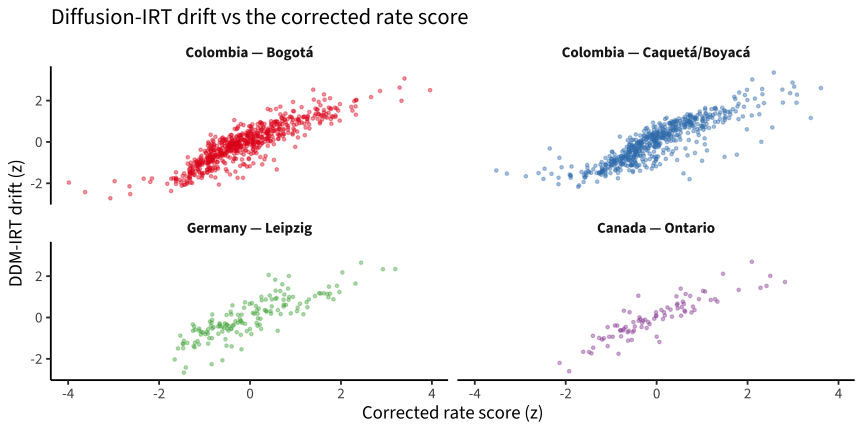
The full model: every trial’s (choice, RT) as a Wiener process, with dataset fixed effects plus run and item random effects on drift (the IRT part), run effects on boundary separation and non-decision time, bias fixed at .5 (~64k trials; item banks are disjoint across sites, so sites are linked by priors, not anchors). Prototyped locally with brms (_fit_sre_ddm.R), then exported to raw Stan (_export_sre_ddm_stan.R) and fit on Sherlock (sherlock_sre_ddm/; 24 cores, 9.5 h, 4 × 500/500). Drift-side parameters converged acceptably (R̂ ≤ 1.06); the run-level non-decision-time hierarchy mixed poorly (R̂ ≈ 1.6) — a known fragility of ndt under a hard global deadline — which cautions against interpreting the ndt estimates but leaves the drift comparison intact.

Code
ddm_file <- here("data/sre_ddm_estimates.rds")
has_ddm <- file.exists(ddm_file)
Code
ddm <- read_rds(ddm_file)

ddm_run <- ddm$run |>
  group_by(dataset) |>
  mutate(drift_z = scale(drift_re)[, 1]) |>
  ungroup()

ddm_first <- sre_first |>
  inner_join(ddm_run |> select(dataset, run_id, drift_z, bs_re, ndt_re),
             by = c("dataset", "run_id"))

ddm_first |>
  pivot_longer(c(age, pa, swr), names_to = "criterion", values_to = "crit") |>
  filter(!is.na(crit)) |>
  group_by(dataset_label, criterion) |>
  filter(n() >= 20) |>
  summarise(n = n(),
            r_rate = cor(score_new, crit),
            r_drift = cor(drift_z, crit),
            r_boundary = cor(bs_re, crit), .groups = "drop") |>
  knitr::kable(digits = 2,
               caption = "Diffusion IRT drift vs corrected rate score: validity")
Diffusion IRT drift vs corrected rate score: validity
dataset_label criterion n r_rate r_drift r_boundary
Colombia — Bogotá age 533 0.60 0.53 -0.18
Colombia — Bogotá pa 365 0.45 0.50 0.09
Colombia — Bogotá swr 198 0.57 0.50 -0.28
Colombia — Caquetá/Boyacá age 567 0.42 0.43 0.17
Colombia — Caquetá/Boyacá pa 557 0.57 0.55 0.12
Germany — Leipzig age 151 0.54 0.44 -0.35
Germany — Leipzig swr 150 0.58 0.62 -0.26
Canada — Ontario age 86 0.39 0.34 -0.27
Canada — Ontario pa 69 0.42 0.43 -0.14
Code
ddm_stab <- sre_scores_pub |>
  filter(dataset == "pilot_uniandes_co_bogota") |>
  inner_join(ddm_run |> select(dataset, run_id, drift_z),
             by = c("dataset", "run_id")) |>
  inner_join(scores_cmp |> select(dataset, run_id, score_new),
             by = c("dataset", "run_id")) |>
  group_by(user_id) |>
  filter(n() >= 2) |>
  arrange(time_started) |>
  summarise(gap = as.numeric(difftime(time_started[2], time_started[1],
                                      units = "days")),
            across(c(drift_z, score_new), list(t1 = ~.x[1], t2 = ~.x[2])),
            .groups = "drop") |>
  filter(gap > 300)

tibble(n_pairs = nrow(ddm_stab),
       rate = cor(ddm_stab$score_new_t1, ddm_stab$score_new_t2),
       ddm_drift = cor(ddm_stab$drift_z_t1, ddm_stab$drift_z_t2)) |>
  knitr::kable(digits = 2,
               caption = "Bogotá 16-month stability: diffusion-IRT drift vs corrected rate")
Bogotá 16-month stability: diffusion-IRT drift vs corrected rate
n_pairs rate ddm_drift
181 0.72 0.56
Code
ddm_first |>
  ggplot(aes(x = score_new, y = drift_z, color = dataset_label)) +
  facet_wrap(vars(dataset_label)) +
  geom_point(alpha = 0.4, size = 0.8, show.legend = FALSE) +
  scale_color_manual(values = dataset_pal) +
  labs(x = "Corrected rate score (z)", y = "DDM-IRT drift (z)",
       title = "Diffusion-IRT drift vs the corrected rate score")

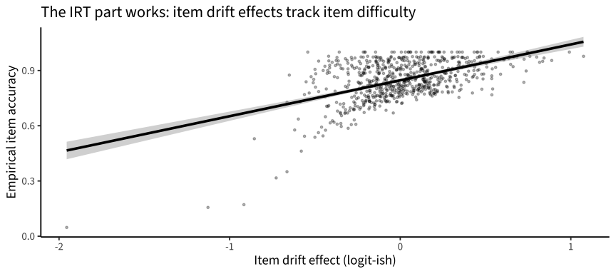
The item side of the model behaves exactly as an IRT model should — item drift effects track empirical item accuracy and (negatively) item RT:

Code
item_emp <- sre |>
  group_by(item_uid) |>
  summarise(accuracy = mean(correct), median_rt = median(rt_s), n = n(),
            .groups = "drop") |>
  filter(n >= 20)

ddm$item |>
  inner_join(item_emp, by = "item_uid") |>
  ggplot(aes(x = drift_re, y = accuracy)) +
  geom_point(alpha = 0.3, size = 0.8) +
  geom_smooth(method = "lm", color = "black") +
  labs(x = "Item drift effect (logit-ish)", y = "Empirical item accuracy",
       title = "The IRT part works: item drift effects track item difficulty")

So the item-level structure that EZ lacked is genuinely recovered here — and person-level drift still underperforms the rate score where they differ. That localizes the problem: it is not missing item information, it is that the diffusion decomposition discards stable, valid between-child variance in time allocation (caution, pacing) that the rate score keeps.

Verdict

1. The timer is mostly honest, but the trial-count rule was aimed at the wrong problem. The first-180-trials filter is a no-op in Germany and Colombia (max 140 trials/run) and bites only in Canada. The real heterogeneity is in time: 20 Canadian runs contain two sequential ~180-s blocks (~360 s of testing scored as one window), and there is a left tail of short runs everywhere (rural Colombia 5th percentile ≈ 87 s of reading time) that the current rule scores as if they had the full window.

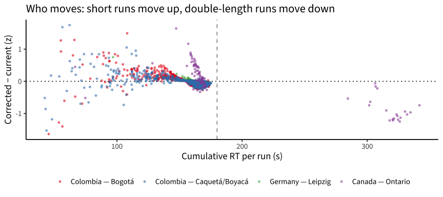
2. Rate normalization changes little in aggregate, a lot for specific kids. Corrected-vs-current r ≈ .997 (DE), .975–.978 (CO), but .82 in Canada (mean |Δ| = 0.45 z there; the double-block runs drop, short runs rise). Validity correlations with age/PA/SWR move by |Δr| ≤ .03 everywhere except Canadian age validity, which improves (.32 → .39); Bogotá 16-month stability ticks up (.70 → .72). So the correction is about fairness of individual scores (especially any longitudinal use of the Canadian data), not about rescuing aggregate structure — which was already fine.

3. Efficiency modeling: a four-rung ladder, and the rate score wins every rung. Every model-based alternative is less valid and/or less stable than the corrected rate score where they differ. The scoreboard below compares all methods on every available metric.

Scoreboard: every method × every metric

Validity columns are n-weighted means of within-dataset correlations (criteria from the hackathon scores: PA/SWR/Vocab/TROG θ, first run per child). Reliability uses the best available estimator per method: odd/even-trial split-half with Spearman–Brown for the trial-computable scores (rate, EZ), model-based empirical reliability for the latent-score methods (zero-fill: mirt EAP rxx; SA/DDM: var(θ̂)/(var(θ̂)+mean(SE²))). Germany test–retest uses levante_data_latest v1_2 (the hackathon subset has no DE repeats): n = 23 pairs at ~3.6 months, rescored per method (DDM would need a full refit — left blank).

Code
# one frame of run-level scores for every method, z within dataset
methods_run <- scores_cmp |>
  select(dataset, run_id, rate = score_new) |>
  full_join(zf |> select(dataset, run_id, zerofill = zf_z),
            by = c("dataset", "run_id")) |>
  full_join(sa_run |> select(dataset, run_id, sa_composite = eff),
            by = c("dataset", "run_id")) |>
  full_join(ez_run |> group_by(dataset) |>
              mutate(ez_drift = scale(drift)[, 1]) |> ungroup() |>
              select(dataset, run_id, ez_drift),
            by = c("dataset", "run_id"))
if (has_ddm) {
  methods_run <- methods_run |>
    full_join(ddm$run |> group_by(dataset) |>
                mutate(ddm_drift = scale(drift_re)[, 1]) |> ungroup() |>
                select(dataset, run_id, ddm_drift),
              by = c("dataset", "run_id"))
}
method_levels <- intersect(
  c("rate", "zerofill", "sa_composite", "ddm_drift", "ez_drift"),
  names(methods_run))

# criteria: age + other language/reading tasks (first run per child)
crit_wide <- sc_all |>
  filter(task_id %in% c("pa", "swr", "vocab", "trog"), !is.na(score)) |>
  first_run() |>
  select(dataset, user_id, task_id, crit_score = score) |>
  pivot_wider(names_from = task_id, values_from = crit_score)

board <- sre_scores_pub |>
  first_run() |>
  select(dataset, user_id, run_id, age) |>
  left_join(crit_wide, by = c("dataset", "user_id")) |>
  inner_join(methods_run, by = c("dataset", "run_id"))

validity <- board |>
  pivot_longer(all_of(method_levels), names_to = "method",
               values_to = "score") |>
  filter(!is.na(score)) |>
  pivot_longer(c(age, pa, swr, vocab, trog), names_to = "criterion",
               values_to = "crit") |>
  filter(!is.na(crit)) |>
  group_by(method, criterion, dataset) |>
  filter(n() >= 20) |>
  summarise(n = n(), r = cor(score, crit), .groups = "drop") |>
  group_by(method, criterion) |>
  summarise(r = weighted.mean(r, n), .groups = "drop") |>
  pivot_wider(names_from = criterion, values_from = r) |>
  select(method, age, pa, swr, vocab, trog)
Code
# split-half (odd/even trials, Spearman-Brown) for rate and EZ
halves <- sre |>
  mutate(half = ifelse(trial_number %% 2 == 0, "even", "odd")) |>
  group_by(dataset, run_id, half) |>
  summarise(rate_h = (sum(correct) - sum(!correct)) / sum(rt_s) * 180,
            n_h = n(), pc_h = mean(correct),
            mrt_h = mean(rt_s[correct & rt_s >= 0.25 & rt_s <= 30]),
            vrt_h = var(rt_s[correct & rt_s >= 0.25 & rt_s <= 30]),
            nc_h = sum(correct), .groups = "drop")

sb <- \(r) 2 * r / (1 + r)
wmean_by_ds <- \(df, x1, x2) df |>
  group_by(dataset) |>
  filter(n() >= 20) |>
  summarise(n = n(), r = cor({{x1}}, {{x2}}, use = "complete.obs"),
            .groups = "drop") |>
  summarise(rel = sb(weighted.mean(r, n))) |> pull(rel)

rate_halves <- halves |>
  filter(n_h >= 5) |>
  select(dataset, run_id, half, rate_h) |>
  pivot_wider(names_from = half, values_from = rate_h) |>
  filter(!is.na(odd), !is.na(even))
rel_rate <- wmean_by_ds(rate_halves, odd, even)

ez_halves <- halves |>
  filter(n_h >= 8, nc_h >= 5, !is.na(vrt_h), vrt_h > 0) |>
  mutate(pc_adj = pmin(pmax(pc_h, 0.5 + 1 / (2 * n_h)), 1 - 1 / (2 * n_h)),
         drift_h = ez_diffusion(pc_adj, vrt_h, mrt_h)$drift) |>
  select(dataset, run_id, half, drift_h) |>
  pivot_wider(names_from = half, values_from = drift_h) |>
  filter(!is.na(odd), !is.na(even))
rel_ez <- wmean_by_ds(ez_halves, odd, even)

# model-based empirical reliability for the latent-score methods
rel_zf <- zf |> distinct(bank, rxx) |>
  left_join(zf |> count(bank), by = "bank") |>
  summarise(rel = weighted.mean(rxx, n)) |> pull(rel)

rel_sa <- sa_run |>
  group_by(dataset) |>
  summarise(err = mean((theta_se / sd(theta))^2) + mean((tau_se / sd(tau))^2),
            tot = var(scale(theta)[, 1] + scale(tau)[, 1]),
            n = n(), .groups = "drop") |>
  summarise(rel = weighted.mean(pmax(0, 1 - err / tot), n)) |> pull(rel)

rel_ddm <- if (has_ddm) ddm$run |>
  group_by(dataset) |>
  summarise(rel = var(drift_re) / (var(drift_re) + mean(drift_se^2)),
            n = n(), .groups = "drop") |>
  summarise(rel = weighted.mean(rel, n)) |> pull(rel) else NA_real_

reliability <- tibble(
  method = c("rate", "zerofill", "sa_composite", "ddm_drift", "ez_drift"),
  reliability = c(rel_rate, rel_zf, rel_sa, rel_ddm, rel_ez),
  rel_type = c("split-half (SB)", "EAP rxx", "model rxx", "model rxx",
               "split-half (SB)"))
Code
# Germany test-retest, levante_data_latest v1_2 (n=23 pairs, ~3.6 months)
de <- read_rds(here("data/sre_de_retest_v1_2.rds"))
de_tr <- de$trials |>
  mutate(correct = as.logical(correct), rt_s = rt_numeric / 1000)

de_scores <- de_tr |>
  group_by(run_id) |>
  summarise(rate = (sum(correct) - sum(!correct)) / sum(rt_s) * 180,
            .groups = "drop")

# zero-fill: score with the hackathon-calibrated DE Rasch model.
# Matrix starts at 0 (unreached AND wrong both 0); set the correct
# responses to 1. Columns follow the model's item order — fscores'
# response.pattern matches by POSITION.
zf_mods <- read_rds(here("data/sre_zerofill_models.rds"))
de_items <- mirt::extract.mirt(zf_mods$de, "itemnames")
de_resp <- matrix(0L, nrow(de_scores), length(de_items),
                  dimnames = list(de_scores$run_id, de_items))
obs <- de_tr |> filter(item_uid %in% de_items, correct)
de_resp[cbind(match(obs$run_id, rownames(de_resp)),
              match(obs$item_uid, de_items))] <- 1L
de_scores$zerofill <- mirt::fscores(zf_mods$de, method = "EAP",
                                    response.pattern = de_resp)[, "F1"]

# EZ per run
de_ez <- de_tr |>
  filter(rt_s >= 0.25, rt_s <= 30) |>
  group_by(run_id) |>
  filter(n() >= 15, sum(correct) >= 10) |>
  summarise(n = n(), pc = mean(correct),
            mrt = mean(rt_s[correct]), vrt = var(rt_s[correct]),
            .groups = "drop") |>
  mutate(pc = pmin(pmax(pc, 0.5 + 1 / (2 * n)), 1 - 1 / (2 * n)),
         ez_drift = ez_diffusion(pc, vrt, mrt)$drift)
de_scores <- de_scores |> left_join(de_ez |> select(run_id, ez_drift),
                                    by = "run_id")

# hierarchical SA refit on the v1_2 DE trials
suppressPackageStartupMessages(library(lme4))
de_lme <- de_tr |> filter(rt_s >= 0.25, rt_s <= 30)
de_acc <- glmer(correct ~ (1 | run_id) + (1 | item_uid), data = de_lme,
                family = binomial, nAGQ = 0)
de_rt <- lmer(log(rt_s) ~ (1 | run_id) + (1 | item_uid), data = de_lme,
              REML = FALSE)
de_sa <- tibble(run_id = rownames(ranef(de_acc)$run_id),
                theta = ranef(de_acc)$run_id[[1]]) |>
  inner_join(tibble(run_id = rownames(ranef(de_rt)$run_id),
                    tau = -ranef(de_rt)$run_id[[1]]), by = "run_id") |>
  mutate(sa_composite = scale(theta)[, 1] + scale(tau)[, 1])
de_scores <- de_scores |> left_join(de_sa |> select(run_id, sa_composite),
                                    by = "run_id")

de_pairs <- de$scores |>
  inner_join(de_scores, by = "run_id") |>
  group_by(user_id) |>
  filter(n() == 2) |>
  arrange(age) |>
  summarise(across(c(rate, zerofill, ez_drift, sa_composite),
                   list(t1 = ~.x[1], t2 = ~.x[2])), .groups = "drop")

retest_de <- tibble(
  method = c("rate", "zerofill", "sa_composite", "ddm_drift", "ez_drift"),
  retest_de = c(cor(de_pairs$rate_t1, de_pairs$rate_t2, use = "complete.obs"),
                cor(de_pairs$zerofill_t1, de_pairs$zerofill_t2,
                    use = "complete.obs"),
                cor(de_pairs$sa_composite_t1, de_pairs$sa_composite_t2,
                    use = "complete.obs"),
                NA_real_,
                cor(de_pairs$ez_drift_t1, de_pairs$ez_drift_t2,
                    use = "complete.obs")))
Code
stab_bog <- sre_scores_pub |>
  filter(dataset == "pilot_uniandes_co_bogota") |>
  inner_join(methods_run, by = c("dataset", "run_id")) |>
  group_by(user_id) |>
  filter(n() >= 2) |>
  arrange(time_started) |>
  summarise(gap = as.numeric(difftime(time_started[2], time_started[1],
                                      units = "days")),
            across(all_of(method_levels), list(t1 = ~.x[1], t2 = ~.x[2])),
            .groups = "drop") |>
  filter(gap > 300)

stability <- tibble(method = method_levels) |>
  rowwise() |>
  mutate(stability_bogota = cor(stab_bog[[paste0(method, "_t1")]],
                                stab_bog[[paste0(method, "_t2")]],
                                use = "complete.obs")) |>
  ungroup()
Code
method_labels <- c(
  rate = "Corrected rate (C − I per 180 s)",
  zerofill = "Zero-filled Rasch (ROAR)",
  sa_composite = "Hierarchical SA composite",
  ddm_drift = "Diffusion-IRT drift",
  ez_drift = "EZ-diffusion drift")

scoreboard <- validity |>
  left_join(reliability, by = "method") |>
  left_join(retest_de, by = "method") |>
  left_join(stability, by = "method") |>
  mutate(method = factor(method, levels = names(method_labels),
                         labels = method_labels)) |>
  arrange(method)

knitr::kable(scoreboard, digits = 2,
             col.names = c("Method", "Age", "PA", "SWR", "Vocab", "TROG",
                           "Reliability", "(estimator)",
                           "DE retest (3.6 mo, n=23)",
                           "Bogotá stability (16 mo, n=181)"),
             caption = "Scoring-method scoreboard. Validity = n-weighted mean within-dataset r; all scores z within dataset.")
Scoring-method scoreboard. Validity = n-weighted mean within-dataset r; all scores z within dataset.
Method Age PA SWR Vocab TROG Reliability (estimator) DE retest (3.6 mo, n=23) Bogotá stability (16 mo, n=181)
Corrected rate (C − I per 180 s) 0.50 0.48 0.57 0.40 0.44 0.83 split-half (SB) 0.83 0.72
Zero-filled Rasch (ROAR) 0.36 0.31 0.52 0.32 0.20 0.88 EAP rxx 0.78 0.72
Hierarchical SA composite 0.42 0.39 0.55 0.46 0.33 0.67 model rxx 0.69 0.68
Diffusion-IRT drift 0.47 0.48 0.49 0.44 0.50 0.87 model rxx NA 0.56
EZ-diffusion drift 0.42 0.45 0.46 0.40 0.47 0.84 split-half (SB) 0.23 0.44

Reading the scoreboard:

  • The corrected rate wins everything that matters for a primary score. Best or tied on age (.50), PA (.48), SWR (.57), best on both repeat-administration metrics (DE 3.6-month retest .83; Bogotá 16-month stability .72), with an honest split-half reliability of .83.
  • One real nuance: speed-purged scores track untimed comprehension slightly better. Diffusion-IRT drift has the best TROG correlation (.50 vs .44 for rate) and drift/SA edge the rate score on Vocab — while the rate score wins on the reading-efficiency-adjacent criteria (SWR, PA, age). That is a sensible division of labor: drift isolates processing efficiency (closer to language knowledge), while the rate score’s pacing component is signal for reading fluency specifically. It validates drift as a research variable without changing the scoring recommendation.
  • Zero-fill’s high nominal reliability (.88) is partly an artifact: the deterministic block of zeros is “reliable” in the rxx sense without being valid — it posts the worst validity column of any method on TROG (.20) and PA (.31). Reliability estimators also aren’t directly comparable across rows (split-half vs model-based).
  • EZ-diffusion’s DE retest of .23 (vs .83 for the rate score on the same 23 children) is the cleanest single demonstration that inverting three summary statistics per run does not produce a usable score.

Item structure is not the missing ingredient: the full diffusion-IRT fit recovers sensible item parameters (item drift effects correlate .52 with item accuracy, −.69 with item median RT) and item information lifts drift stability from .44 (EZ) to .56 — but still far short of .72. Validity tells the same story (e.g. Bogotá age r: rate .60, DDM drift .53; DE age: .54 vs .44), with only scattered small wins for model-based scores (DE SWR: DDM .62 vs rate .58). The diagnosis: SRE’s net rate is the behaviorally meaningful quantity — it bundles decision efficiency and stable individual differences in pacing/caution, and every decomposition that strips the latter out throws away true-score variance. The site-dependent ability–speed correlation (≈ 0 in DE/Canada, −.52 in rural CO, where fast = guessing) additionally means no fixed recombination of decomposed parts travels across sites.

Recommendations for the DCC:

  • Adopt rate normalization now (patch below). It fixes the Canadian double-block and short-run distortions at zero modeling cost and is what the ROAR “net correct in 3 minutes” score means.
  • If a measurement model is wanted, the next step is an offset-Poisson / Rasch-Poisson counts GLMM (net-correct count with offset(log(time)), corpus fixed effects, child random effects) — it is rate normalization with standard errors and corpus adjustment, not a new scoring philosophy.
  • Diffusion IRT is now tested, not just argued against: don’t use it for the primary SRE score. The full hierarchical Wiener fit (9.5 h on Sherlock) yields drift scores that are less stable (.56 vs .72) and mostly less valid than the rate score. The decomposition (drift vs boundary vs ndt) remains available in data/sre_ddm_estimates.rds for substantive questions about speed–accuracy tradeoff and its development — boundary separation declines with age in every dataset — but that is a research variable, not a score.
  • Use RT for data quality regardless: sub-second responses sit at chance and range from 3% of trials (DE) to 31% (rural CO). A fast-guess flag (e.g. proportion of RT < 1 s) is a cheap, useful run-level QC covariate.
Proposed patch to levantemodels::score_sre():

score_sre <- \(trial_data_task, dataset) {
  trial_data_task |>
    group_by(.data$run_id) |>
    summarise(elapsed = sum(.data$rt_numeric, na.rm = TRUE) / 1000,
              net = sum(.data$correct) - sum(!.data$correct)) |>
    filter(.data$elapsed >= 30) |>
    mutate(score = scale(.data$net / .data$elapsed * 180)[, 1],
           score_type = "guessing_adjusted_rate_scaled") |>
    select(-"elapsed", -"net")
}