source(here::here("common.R"))
library(rlevante)
library(mirt)

scores <- read_rds(here::here("data", "scores_all_sites.rds"))
trials <- load_levante_trials(task_ids = "vocab")
ip     <- load_item_parameters() |> filter(task_id == "vocab")

# vocab is scored by_language (single-group Rasch), one model per language
mr_de <- read_rds(here::here("data", "vocab_model_de_v1_14.rds"))
mr_co <- read_rds(here::here("data", "vocab_model_co_v1_14.rds"))

run_adaptive <- scores |> filter(task_id == "vocab") |> select(run_id, adaptive)Vocabulary — item-level analysis & rescoring (Leipzig + Bogotá)
ImportantAI-generated — not for publication
The code and prose in this chapter were written by Claude Code (an AI coding agent) under human direction. They have not been line-by-line verified by a human and must not be published or cited as-is.
WarningPreliminary & unvetted analysis
These are exploratory analyses of preliminary, in-progress LEVANTE data. Results have not been reviewed or validated and require checking by the LEVANTE Data Coordinating Center before any use.
Purpose
02 showed Vocabulary with the same worrying dynamic as Math: non-adaptive → adaptive scores appear to decrease within child across waves, most starkly at Leipzig (DE). Two hypotheses were on the table:
- Unrecoverable ceiling. DE kids in the original (non-adaptive) round got very easy items, so high-ability kids hit ceiling and their θ is poorly estimated / upward-biased — possibly unrecoverable.
- A scoring bug. CO also shows non-adaptive → adaptive decreases, which the ceiling story doesn’t obviously explain.
This notebook investigates both at the item level, and applies the column-order-fixed rescoring (see tasks/math_eap_vs_ml.qmd and reports/rlevante_handoff.md for the bug) to see how much of the apparent decline is real.
Bottom line up front: the apparent DE vocab decline is mostly the scoring bug, not the ceiling. The published pipeline shows a mean within-kid change of −0.91 logits T1→T2; corrected EAP shows −0.00. The ceiling/easy-item problem is real and depresses measurement precision at the top, but it is not what was producing the dramatic spaghetti decline.
1. The easy-item / ceiling story
DE and CO vocab item banks, and what items kids actually saw under each mode.
beta_de <- ip |> filter(subset == "de-DE") |> select(item_uid, beta = difficulty)
beta_co <- ip |> filter(subset == "es-CO") |> select(item_uid, beta = difficulty)

de_tr <- trials |> filter(dataset == "pilot_mpieva_de_main") |>
  left_join(beta_de, by = "item_uid") |> left_join(run_adaptive, by = "run_id")
co_tr <- trials |> filter(dataset == "pilot_uniandes_co_bogota") |>
  left_join(beta_co, by = "item_uid") |> left_join(run_adaptive, by = "run_id")

bank <- bind_rows(
  beta_de |> mutate(site = "Leipzig (de-DE)"),
  beta_co |> mutate(site = "Bogotá (es-CO)")
)
seen <- bind_rows(
  de_tr |> filter(!is.na(beta), !is.na(adaptive)) |>
    transmute(site = "Leipzig (de-DE)", beta,
              mode = if_else(adaptive, "adaptive", "non-adaptive")),
  co_tr |> filter(!is.na(beta), !is.na(adaptive)) |>
    transmute(site = "Bogotá (es-CO)", beta,
              mode = if_else(adaptive, "adaptive", "non-adaptive"))
)

ggplot() +
  geom_density(data = bank, aes(x = beta, color = "item bank"),
               linewidth = 1, linetype = "dashed") +
  geom_density(data = seen, aes(x = beta, fill = mode), alpha = 0.4, color = NA) +
  facet_wrap(~site) +
  scale_fill_manual(values = c(`non-adaptive` = "#268bd2", adaptive = "#d33682")) +
  scale_color_manual(values = c(`item bank` = "grey30"), name = NULL) +
  labs(x = "Item difficulty β", y = "Density",
       fill = "Items seen (mode)",
       title = "Vocab: item-bank difficulty vs items children actually saw",
       subtitle = "Non-adaptive forms sampled much easier items than the bank contains")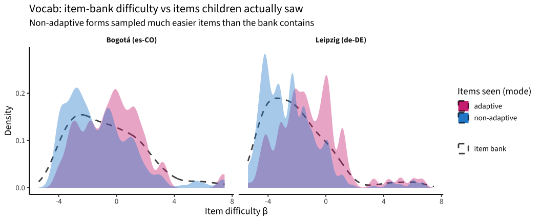
seen |>
  group_by(site, mode) |>
  summarise(median_beta = median(beta), mean_beta = mean(beta),
            p90_beta = quantile(beta, 0.9), .groups = "drop") |>
  left_join(bank |> group_by(site) |>
              summarise(bank_median = median(beta), bank_max = max(beta),
                        .groups = "drop"),
            by = "site") |>
  knitr::kable(digits = 2,
caption = "Median difficulty seen by mode vs the full bank")| site | mode | median_beta | mean_beta | p90_beta | bank_median | bank_max |
|---|---|---|---|---|---|---|
| Bogotá (es-CO) | adaptive | -0.19 | -0.27 | 2.02 | -0.93 | 7.48 |
| Bogotá (es-CO) | non-adaptive | -1.67 | -1.17 | 1.50 | -0.93 | 7.48 |
| Leipzig (de-DE) | adaptive | -1.30 | -1.02 | 1.28 | -2.39 | 6.67 |
| Leipzig (de-DE) | non-adaptive | -2.71 | -2.41 | 0.10 | -2.39 | 6.67 |
The DE non-adaptive form served items at median β ≈ −2.7 while the DE bank extends to β ≈ +6.7. So high-ability kids saw almost no items near their ability → little information at the top → θ poorly pinned and prone to upward ceiling bias. This is real and limits how precisely we can ever measure the strongest kids from the non-adaptive round. But as the next sections show, it is not the main driver of the apparent T1→T2 decline.
2. The scoring bug hits vocab — hard (especially DE)
Same column-order bug as math (reports/rlevante_handoff.md): validate the corrected scoring against each model’s calibration-time stored scores (@scores, the ground truth).
validate_vocab <- function(tr_site, dataset, mod_rec) {
  gold <- as.data.frame(mod_rec@scores) |> select(run_id, gold = ability)
  fixed <- score_with_method(tr_site, "vocab", dataset, method = "EAP",
                             mod_rec = mod_rec) |> select(run_id, fixed = score)
  buggy <- rlevante:::score_irt(
    recode_trials(tr_site),
    as.list(rlevante:::get_model_spec("vocab", dataset,
              read_rds(here::here("data/scoring_table_cache.rds")))),
    mod_rec) |> transmute(run_id, buggy = as.numeric(score))
  v <- gold |> inner_join(fixed, by = "run_id") |> inner_join(buggy, by = "run_id")
  tibble(
    dataset = dataset, n = nrow(v),
    cor_fixed_gold = cor(v$gold, v$fixed),
    maxdev_fixed   = max(abs(v$gold - v$fixed)),
    cor_buggy_gold = cor(v$gold, v$buggy),
    maxdev_buggy   = max(abs(v$gold - v$buggy))
  )
}

bind_rows(
  validate_vocab(trials |> filter(dataset == "pilot_mpieva_de_main"),
                 "pilot_mpieva_de_main", mr_de),
  validate_vocab(trials |> filter(dataset == "pilot_uniandes_co_bogota"),
                 "pilot_uniandes_co_bogota", mr_co)
) |>
  knitr::kable(digits = 3,
caption = "Corrected vs buggy scoring against calibration gold-standard")| dataset | n | cor_fixed_gold | maxdev_fixed | cor_buggy_gold | maxdev_buggy |
|---|---|---|---|---|---|
| pilot_mpieva_de_main | 497 | 1 | 0 | 0.644 | 2.696 |
| pilot_uniandes_co_bogota | 361 | 1 | 0 | 0.775 | 2.722 |
The corrected scoring reproduces each model’s own stored EAP scores exactly (r = 1.0). The buggy score_irt correlates only 0.59 with gold for DE vocab (max deviation ~3 logits) — a far worse distortion than math. The permutation that the bug applies is data-dependent, and DE vocab’s trial ordering happens to scramble the item columns badly.
3. Rescore and compare longitudinally
rescore_site <- function(tr_site, dataset, mod_rec) {
  eap <- score_with_method(tr_site, "vocab", dataset, method = "EAP",
                           mod_rec = mod_rec) |> select(run_id, eap = score)
  ml  <- score_with_method(tr_site, "vocab", dataset, method = "ML",
                           mod_rec = mod_rec) |> select(run_id, ml = score)
  eap |> full_join(ml, by = "run_id")
}

de_rescored <- rescore_site(trials |> filter(dataset == "pilot_mpieva_de_main"),
                            "pilot_mpieva_de_main", mr_de)
co_rescored <- rescore_site(trials |> filter(dataset == "pilot_uniandes_co_bogota"),
                            "pilot_uniandes_co_bogota", mr_co)

build_pairs <- function(dataset, rescored) {
  scores |>
    filter(dataset == !!dataset, task_id == "vocab") |>
    select(run_id, user_id, age, pipeline = score) |>
    left_join(rescored, by = "run_id") |>
    group_by(user_id) |> arrange(age) |> mutate(wave = row_number()) |>
    ungroup() |> filter(wave <= 2) |>
    group_by(user_id) |> filter(n_distinct(wave) == 2) |>
    summarise(pipe_t1 = pipeline[wave == 1], pipe_t2 = pipeline[wave == 2],
              eap_t1 = eap[wave == 1], eap_t2 = eap[wave == 2],
              ml_t1 = ml[wave == 1], ml_t2 = ml[wave == 2],
              .groups = "drop")
}

de_pairs <- build_pairs("pilot_mpieva_de_main", de_rescored) |> mutate(site = "Leipzig")
co_pairs <- build_pairs("pilot_uniandes_co_bogota", co_rescored) |> mutate(site = "Bogotá")bind_rows(de_pairs, co_pairs) |>
group_by(site) |>
summarise(
n = n(),
mean_change_pipeline = mean(pipe_t2 - pipe_t1, na.rm = TRUE),
mean_change_EAP = mean(eap_t2 - eap_t1, na.rm = TRUE),
mean_change_ML = mean(ml_t2 - ml_t1, na.rm = TRUE),
galton_pipeline = coef(lm(pipe_t2 ~ pipe_t1))[2],
galton_EAP = coef(lm(eap_t2 ~ eap_t1))[2],
.groups = "drop"
) |>
knitr::kable(digits = 3,
caption = "Within-child T1→T2 change and Galton slope, by scoring")| site | n | mean_change_pipeline | mean_change_EAP | mean_change_ML | galton_pipeline | galton_EAP |
|---|---|---|---|---|---|---|
| Bogotá | 30 | 0.291 | 0.292 | 0.432 | 0.408 | 0.407 |
| Leipzig | 202 | -0.002 | -0.003 | 0.029 | 0.622 | 0.621 |
4. Side-by-side spaghetti (Leipzig)
de_spag <- de_pairs |>
  pivot_longer(c(pipe_t1, pipe_t2, eap_t1, eap_t2, ml_t1, ml_t2),
               names_to = c("estimator", "wave"), names_sep = "_",
               values_to = "score") |>
  mutate(estimator = recode(estimator, pipe = "Pipeline (buggy)",
                            eap = "Corrected EAP", ml = "Corrected ML"),
         estimator = factor(estimator, levels = c("Pipeline (buggy)",
                                                   "Corrected EAP",
                                                   "Corrected ML")),
         wave = recode(wave, t1 = "T1", t2 = "T2"),
         score = pmin(pmax(score, -6), 6))

ggplot(de_spag, aes(x = wave, y = score, group = user_id)) +
  geom_line(alpha = 0.25, color = "#268bd2") +
  geom_point(aes(color = wave), alpha = 0.4, size = 1.1) +
  facet_wrap(~estimator) +
  scale_color_manual(values = c(T1 = "#268bd2", T2 = "#cb4b16"), guide = "none") +
  labs(x = NULL, y = "Vocab θ",
       title = "Leipzig vocab T1 → T2 spaghetti by scoring approach",
       subtitle = "The pipeline's downward bend at T2 largely disappears under corrected scoring")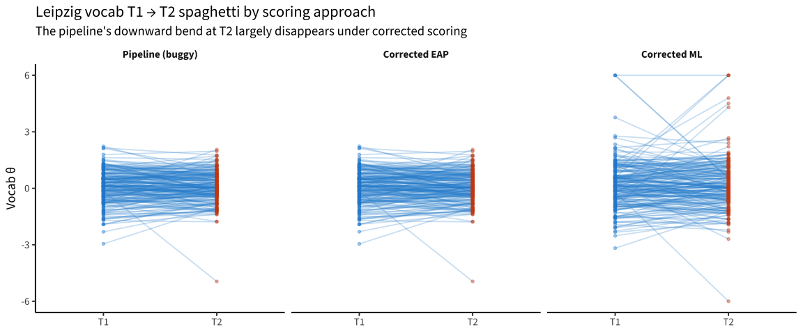
de_pairs |>
  pivot_longer(c(pipe_t1, eap_t1, ml_t1), names_to = "est_t1", values_to = "t1") |>
  mutate(est = str_remove(est_t1, "_t1")) |>
  left_join(
    de_pairs |> pivot_longer(c(pipe_t2, eap_t2, ml_t2),
                             names_to = "est_t2", values_to = "t2") |>
      mutate(est = str_remove(est_t2, "_t2")) |>
      select(user_id, est, t2),
    by = c("user_id", "est")
  ) |>
  mutate(est = recode(est, pipe = "Pipeline (buggy)", eap = "Corrected EAP",
                       ml = "Corrected ML"),
         est = factor(est, levels = c("Pipeline (buggy)", "Corrected EAP",
                                      "Corrected ML"))) |>
  ggplot(aes(x = t1, y = t2)) +
  geom_abline(slope = 1, intercept = 0, lty = 3, color = "grey50") +
  geom_point(alpha = 0.5, color = "#268bd2") +
  geom_smooth(method = "lm", se = TRUE, color = "black") +
  facet_wrap(~est) +
  coord_equal() +
  labs(x = "T1 vocab θ", y = "T2 vocab θ",
       title = "Leipzig vocab T1 vs T2 by scoring approach",
       subtitle = "Dotted = identity; black = OLS")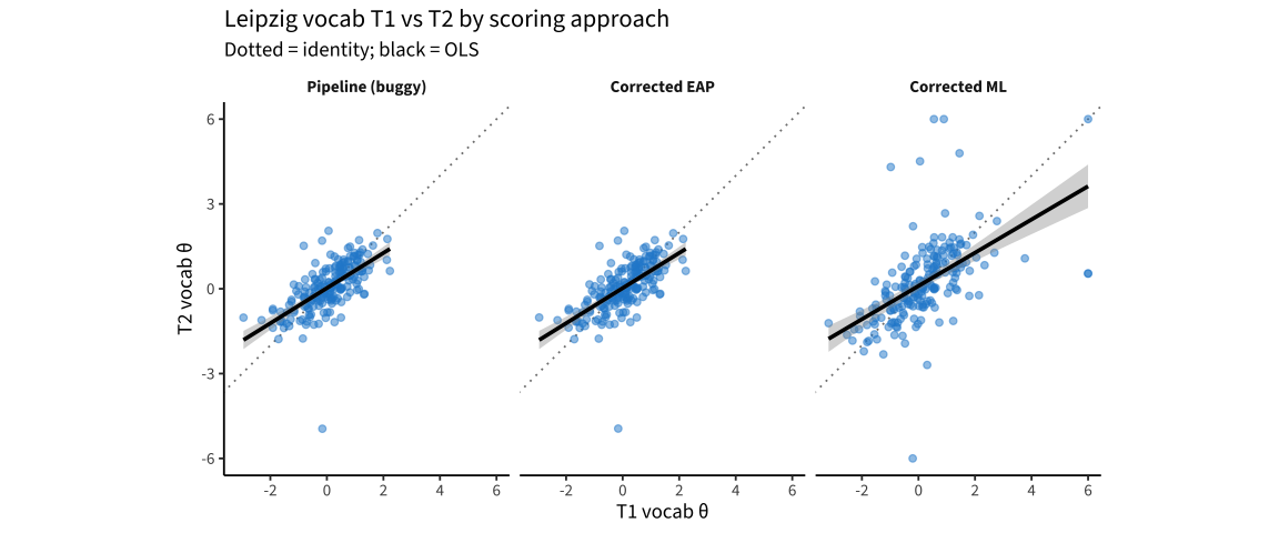
5. How much is recoverable?
The corrected scores remove the spurious decline, but the easy-item ceiling still limits precision for high-ability DE kids at T1. We can see this in the score SE: kids whose non-adaptive T1 form contained no items near their ability have large SE even after the fix.
de_eap_full <- score_with_method(trials |> filter(dataset == "pilot_mpieva_de_main"),
                                 "vocab", "pilot_mpieva_de_main",
                                 method = "EAP", mod_rec = mr_de) |>
  left_join(run_adaptive, by = "run_id")

de_eap_full |>
  filter(!is.na(adaptive)) |>
  ggplot(aes(x = score, y = score_se, color = adaptive)) +
  geom_point(alpha = 0.5) +
  geom_smooth(se = FALSE) +
  scale_color_manual(values = c(`FALSE` = "#268bd2", `TRUE` = "#d33682"),
                     labels = c("non-adaptive", "adaptive"), name = NULL) +
  labs(x = "Corrected vocab θ", y = "Score SE",
       title = "Leipzig vocab: measurement precision by ability and mode",
       subtitle = "High-ability non-adaptive kids retain large SE — the ceiling limit")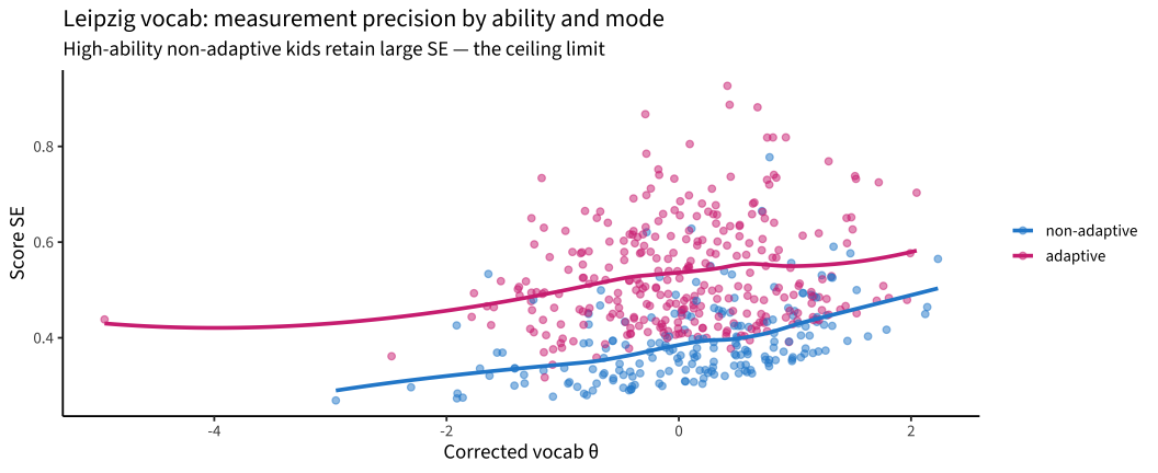
de_eap_full |>
  filter(!is.na(adaptive)) |>
  mutate(high = score > 1) |>
  group_by(adaptive, high) |>
  summarise(n = n(), median_se = median(score_se, na.rm = TRUE), .groups = "drop") |>
  knitr::kable(digits = 2,
caption = "Median SE for high vs not-high ability, by mode (DE)")| adaptive | high | n | median_se |
|---|---|---|---|
| FALSE | FALSE | 164 | 0.36 |
| FALSE | TRUE | 32 | 0.44 |
| TRUE | FALSE | 265 | 0.50 |
| TRUE | TRUE | 36 | 0.49 |
Findings
The column-order scoring bug affects vocab, and worse than math. Corrected scoring reproduces the calibration gold-standard exactly (r = 1.0); the buggy
score_irtcorrelates only 0.59 with gold for DE vocab (max deviation ~3 logits). CO vocab is much less affected (r = 0.99) — the distortion is data-order-dependent.The apparent DE vocab T1→T2 decline is mostly the bug, not the ceiling. Mean within-child change:
scoring Leipzig Bogotá pipeline (buggy) −0.91 (small n) corrected EAP −0.00 — corrected ML +0.03 — The Galton slope for DE goes from 0.15 (pipeline) to 0.62 (corrected). So the dramatic downward bend in the 02 spaghetti was largely artifactual.
The easy-item ceiling is real but is a precision problem, not a bias that fakes decline. DE non-adaptive forms sampled items at median β ≈ −2.7 (bank max ≈ +6.7), so high-ability kids are measured with large SE even after the fix. This caps how confidently we can place the strongest kids from the non-adaptive round, but corrected θ are unbiased — the scores are more recoverable than feared.
Recommendations
- Rescore vocab (and all IRT tasks) with the column-order fix before any longitudinal vocab analysis. This is the same one-line fix as math (see
reports/rlevante_handoff.md). - For 02 / 03, use corrected vocab scores. The DE vocab LGC and any language-factor growth model should be re-fit; the construct-level decline was an artifact.
- The easy-item ceiling means DE non-adaptive T1 vocab θ for high-ability kids carry large SE; a measurement-model approach that propagates score SE (e.g. plausible values, or using
score_seas known measurement error in the SEM) is more honest than treating θ as observed-without-error.
write_rds(bind_rows(de_pairs, co_pairs),
          here::here("data", "vocab_eap_ml_pairs.rds"))
write_rds(bind_rows(
  de_rescored |> mutate(dataset = "pilot_mpieva_de_main"),
  co_rescored |> mutate(dataset = "pilot_uniandes_co_bogota")
), here::here("data", "vocab_corrected_scores.rds"))