source(here::here("common.R"))

scores <- read_rds(here::here("data", "scores_all_sites.rds"))
trials <- load_levante_trials(task_ids = "swr")ROAR-Word (SWR) — trial-level investigation
ImportantAI-generated — not for publication
The code and prose in this chapter were written by Claude Code (an AI coding agent) under human direction. They have not been line-by-line verified by a human and must not be published or cited as-is.
WarningPreliminary & unvetted analysis
These are exploratory analyses of preliminary, in-progress LEVANTE data. Results have not been reviewed or validated and require checking by the LEVANTE Data Coordinating Center before any use.
Purpose
01 flagged a cluster of ~40 children in Bogotá whose ROAR-Word ability_cat score floored at θ = −6 with score_se = 37. Initial guess was truncated CAT runs, but those kids attempted ~120 items (a full administration). This notebook digs into the trial-level data to figure out what those kids were actually doing.
ROAR-Word is a 2-alternative forced-choice lexical decision (real word vs. non-word) → chance = 50%.
Score vs accuracy: where does θ = −6 come from?
run_accuracy <- trials |>
  group_by(dataset, dataset_label, run_id, user_id) |>
  summarise(
    n_trials      = n(),
    n_correct     = sum(correct, na.rm = TRUE),
    pct_correct   = mean(correct, na.rm = TRUE),
    median_rt_ms  = median(rt_numeric, na.rm = TRUE),
    mean_rt_ms    = mean(rt_numeric, na.rm = TRUE),
    .groups       = "drop"
  )

# Join scores
run_summary <- scores |>
  filter(task_id == "swr") |>
  select(dataset, dataset_label, run_id, user_id, age, score, score_se, adaptive) |>
  inner_join(run_accuracy, by = c("dataset", "dataset_label",
                                  "run_id", "user_id"))

run_summary |>
  filter(dataset == "pilot_uniandes_co_bogota") |>
  ggplot(aes(x = pct_correct, y = score)) +
  geom_hline(yintercept = -6, lty = 3, color = "red") +
  geom_vline(xintercept = 0.5, lty = 3, color = "grey50") +
  geom_point(aes(color = age), alpha = 0.6) +
  scale_color_viridis_c() +
  labs(x = "Trial-level accuracy (% correct)",
       y = "Final IRT θ score",
       title = "ROAR-Word score vs trial accuracy (Bogotá)",
       subtitle = "Red = score floor; grey = chance (50% on 2AFC)") +
  theme(legend.position = "right")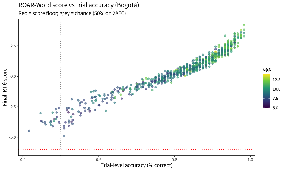
Categorize runs by trial accuracy
run_summary <- run_summary |>
  mutate(category = case_when(
    pct_correct >= 0.75 ~ "strong (≥75%)",
    pct_correct >= 0.6  ~ "moderate (60–75%)",
    pct_correct >= 0.5  ~ "near chance (50–60%)",
    pct_correct >= 0.4  ~ "at chance (40–50%)",
    TRUE                ~ "below chance (<40%)"
  ) |> factor(levels = c("strong (≥75%)", "moderate (60–75%)",
                          "near chance (50–60%)",
                          "at chance (40–50%)",
                          "below chance (<40%)")))

run_summary |>
  filter(dataset == "pilot_uniandes_co_bogota") |>
  count(category, name = "n_runs") |>
  mutate(pct = n_runs / sum(n_runs) * 100) |>
knitr::kable(digits = 1)| category | n_runs | pct |
|---|---|---|
| strong (≥75%) | 559 | 78.1 |
| moderate (60–75%) | 94 | 13.1 |
| near chance (50–60%) | 44 | 6.1 |
| at chance (40–50%) | 19 | 2.7 |
run_summary |>
  filter(dataset == "pilot_uniandes_co_bogota") |>
  ggplot(aes(x = age, fill = category)) +
  geom_histogram(binwidth = 0.5) +
  scale_fill_brewer(palette = "RdYlGn", direction = -1) +
  labs(x = "Age (years)", y = "Runs",
       title = "ROAR-Word run categories by age (Bogotá)",
       fill = NULL) +
  theme(legend.position = "right")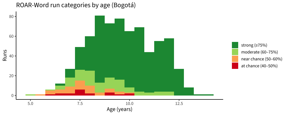
RT distributions: are below-chance kids button-mashing?
trials |>
  filter(dataset == "pilot_uniandes_co_bogota") |>
  inner_join(run_summary |>
               select(run_id, category),
             by = "run_id") |>
  filter(!is.na(rt_numeric), rt_numeric > 0, rt_numeric < 30000) |>
  ggplot(aes(x = rt_numeric, fill = category)) +
  geom_density(alpha = 0.5) +
  scale_x_log10() +
  facet_wrap(~category, ncol = 5) +
  scale_fill_brewer(palette = "RdYlGn", direction = -1, guide = "none") +
  geom_vline(xintercept = 300, lty = 3, color = "red") +
  labs(x = "Trial RT (ms, log)", y = "Density",
       title = "RT distributions by accuracy category (Bogotá)",
       subtitle = "Red = 300 ms cutoff (faster than plausible reading time)")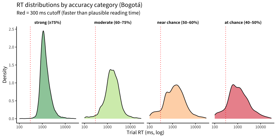
run_summary |>
  filter(dataset == "pilot_uniandes_co_bogota") |>
  group_by(category) |>
  summarise(
    n_runs       = n(),
    median_rt    = median(median_rt_ms),
    mean_rt      = mean(median_rt_ms),
    pct_fast_rt  = mean(median_rt_ms < 500) * 100,
    pct_very_fast = mean(median_rt_ms < 300) * 100
  ) |>
  knitr::kable(digits = 1,
               col.names = c("Category", "N runs", "Median of medians (ms)",
                             "Mean median (ms)",
                             "% runs with median RT < 500ms",
"% runs with median RT < 300ms"))| Category | N runs | Median of medians (ms) | Mean median (ms) | % runs with median RT < 500ms | % runs with median RT < 300ms |
|---|---|---|---|---|---|
| strong (≥75%) | 559 | 1243.5 | 1304.0 | 0 | 0 |
| moderate (60–75%) | 94 | 1455.5 | 1669.7 | 0 | 0 |
| near chance (50–60%) | 44 | 1197.2 | 1299.3 | 0 | 0 |
| at chance (40–50%) | 19 | 845.0 | 1098.2 | 0 | 0 |
Response-side bias: are they pressing only one key?
For each run, what proportion of responses are “yes/real word” answers? If a kid is just pressing one button, this will be near 0 or near 1.
response_bias <- trials |>
  filter(dataset == "pilot_uniandes_co_bogota") |>
  mutate(answer_clean = str_to_lower(str_trim(as.character(answer))),
         resp_clean   = str_to_lower(str_trim(as.character(response)))) |>
  group_by(run_id) |>
  summarise(
    n_resp        = sum(!is.na(resp_clean)),
    n_unique_resp = n_distinct(resp_clean, na.rm = TRUE),
    pct_response_a = mean(resp_clean == names(sort(table(resp_clean),
                                                    decreasing = TRUE))[1],
                          na.rm = TRUE),
    .groups = "drop"
  )

run_summary |>
  filter(dataset == "pilot_uniandes_co_bogota") |>
  left_join(response_bias, by = "run_id") |>
  ggplot(aes(x = pct_response_a, y = score, color = category)) +
  geom_hline(yintercept = -6, lty = 3, color = "red") +
  geom_vline(xintercept = c(0.5, 1.0), lty = 3, color = "grey60") +
  geom_point(alpha = 0.5) +
  scale_color_brewer(palette = "RdYlGn", direction = -1) +
  labs(x = "Proportion of responses on the modal response value",
       y = "IRT score",
       title = "Score vs one-key-pressing tendency",
       subtitle = "1.0 on x means the kid pressed the same response every trial",
       color = NULL) +
  theme(legend.position = "right")
Trial-by-trial: do floor kids ever respond carefully?
Plot per-trial RTs across the run for a sample of floor-score kids.
floor_runs <- run_summary |>
  filter(dataset == "pilot_uniandes_co_bogota", score < -3) |>
  pull(run_id)

set.seed(7)
sample_floor_runs <- sample(floor_runs, min(9, length(floor_runs)))

trials |>
  filter(run_id %in% sample_floor_runs) |>
  filter(!is.na(rt_numeric), rt_numeric > 0, rt_numeric < 10000) |>
  ggplot(aes(x = trial_number, y = rt_numeric, color = correct)) +
  geom_point(alpha = 0.6) +
  geom_hline(yintercept = 300, lty = 3, color = "red") +
  facet_wrap(~run_id, scales = "free", ncol = 3) +
  scale_color_manual(values = c(`TRUE` = "darkgreen", `FALSE` = "firebrick"),
                     na.value = "grey60") +
  labs(x = "Trial number", y = "RT (ms)",
       title = "RT timeline for floor-score kids (sample of 9)",
       color = "Correct")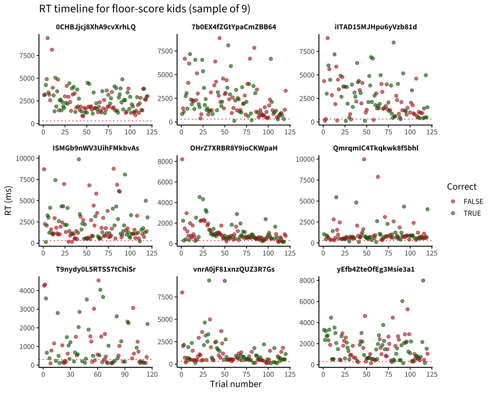
Running CAT theta over trials
The trial-level theta_estimate shows the CAT’s running ability estimate. For floor-score kids it should bottom out fast.
trials |>
  filter(run_id %in% sample_floor_runs) |>
  ggplot(aes(x = trial_number, y = theta_estimate)) +
  geom_ribbon(aes(ymin = theta_estimate - theta_se,
                  ymax = theta_estimate + theta_se),
              fill = "grey80", alpha = 0.5) +
  geom_line(color = "steelblue") +
  geom_point(aes(color = correct), size = 0.7) +
  geom_hline(yintercept = c(-6, 0), lty = 3, color = "grey50") +
  facet_wrap(~run_id, ncol = 3) +
  scale_color_manual(values = c(`TRUE` = "darkgreen", `FALSE` = "firebrick"),
                     na.value = "grey60") +
  labs(x = "Trial number", y = "Running θ estimate",
       title = "CAT running theta for floor-score kids",
       color = "Correct")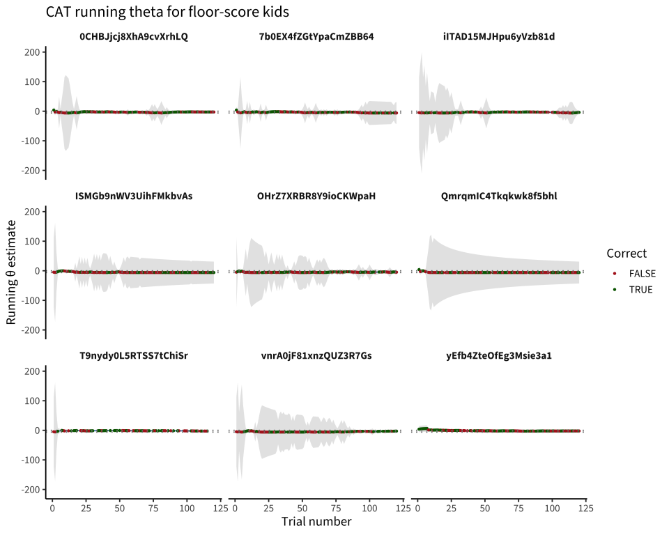
Item difficulty: are they getting easier items as they fail?
ROAR-Word CAT should serve easier items when the running θ drops. Let’s see.
trials |>
  filter(run_id %in% sample_floor_runs) |>
  ggplot(aes(x = trial_number, y = difficulty, color = correct)) +
  geom_point(alpha = 0.6) +
  geom_smooth(aes(group = run_id), method = "loess", se = FALSE,
              color = "steelblue") +
  facet_wrap(~run_id, ncol = 3) +
  scale_color_manual(values = c(`TRUE` = "darkgreen", `FALSE` = "firebrick"),
                     na.value = "grey60") +
  labs(x = "Trial number", y = "Item difficulty",
       title = "Item difficulty trajectory for floor-score kids",
       color = "Correct")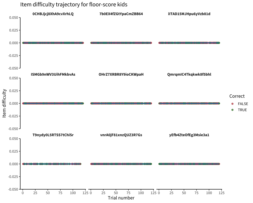
Compare to high scorers
set.seed(7)
high_runs <- run_summary |>
  filter(dataset == "pilot_uniandes_co_bogota",
         category == "strong (≥75%)") |>
  pull(run_id)
sample_high_runs <- sample(high_runs, 9)

trials |>
  filter(run_id %in% sample_high_runs) |>
  ggplot(aes(x = trial_number, y = theta_estimate)) +
  geom_ribbon(aes(ymin = theta_estimate - theta_se,
                  ymax = theta_estimate + theta_se),
              fill = "grey80", alpha = 0.5) +
  geom_line(color = "steelblue") +
  geom_point(aes(color = correct), size = 0.7) +
  geom_hline(yintercept = c(-6, 0), lty = 3, color = "grey50") +
  facet_wrap(~run_id, ncol = 3) +
  scale_color_manual(values = c(`TRUE` = "darkgreen", `FALSE` = "firebrick"),
                     na.value = "grey60") +
  labs(x = "Trial number", y = "Running θ estimate",
       title = "CAT running theta for HIGH-scoring kids (comparison)",
       color = "Correct")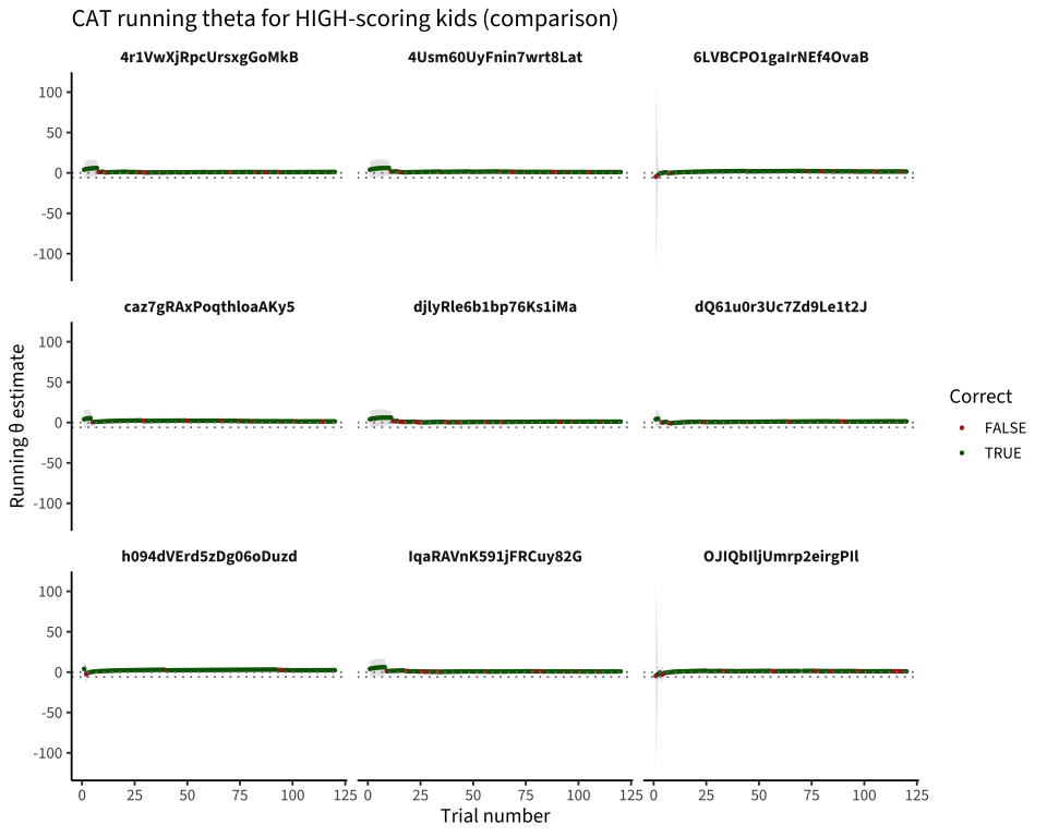
How does floor-vs-not look in Leipzig and Western-CA?
run_summary |>
  group_by(dataset_label) |>
  summarise(
    n          = n(),
    n_floor    = sum(score < -3),
    pct_floor  = mean(score < -3) * 100,
    n_below_chance = sum(pct_correct < 0.4),
    .groups = "drop"
  ) |>
knitr::kable(digits = 1)| dataset_label | n | n_floor | pct_floor | n_below_chance |
|---|---|---|---|---|
| Colombia — Bogotá | 716 | 28 | 3.9 | 0 |
| Colombia — Caquetá/Boyacá | 599 | 86 | 14.4 | 0 |
| Germany — Leipzig | 183 | NA | NA | 0 |
| Canada — Ontario | 112 | 7 | 6.2 | 0 |
Filter proposal
Based on the above, candidate exclusion rules for ROAR-Word at the run level:
- Trial accuracy below chance (< 40%) → likely random responding / non-engagement.
- Median RT < 500ms → too fast to plausibly read words.
- Response-side bias > 95% (kid pressed same key on > 95% of trials).
run_summary_co <- run_summary |>
  filter(dataset == "pilot_uniandes_co_bogota") |>
  left_join(response_bias, by = "run_id") |>
  mutate(
    flag_below_chance = pct_correct < 0.4,
    flag_fast_rt      = median_rt_ms < 500,
    flag_one_key      = pct_response_a > 0.95
  )

run_summary_co |>
  count(flag_below_chance, flag_fast_rt, flag_one_key,
        name = "n_runs") |>
  arrange(desc(n_runs)) |>
knitr::kable()| flag_below_chance | flag_fast_rt | flag_one_key | n_runs |
|---|---|---|---|
| FALSE | FALSE | NA | 716 |
run_summary_co |>
  mutate(any_flag = flag_below_chance | flag_fast_rt | flag_one_key) |>
  group_by(any_flag) |>
  summarise(
    n = n(),
    median_score = median(score),
    mean_score = mean(score),
    pct_at_floor = mean(score < -3) * 100,
    .groups = "drop"
  ) |>
knitr::kable(digits = 2)| any_flag | n | median_score | mean_score | pct_at_floor |
|---|---|---|---|---|
| NA | 716 | 0.8 | 0.59 | 3.91 |
Verdict
cat("- The 40 Bogotá floor-score kids are scoring at chance or below ",
    "(37–46% on a 2AFC task). They aren't broken IRT runs — they completed",
    " ~120 trials but the model can't extract a reliable ability estimate ",
    "below the floor.\n",
    "- A subset show fast median RTs (< 500 ms) consistent with rushing or ",
    "non-engagement; another subset show slower RTs and look like genuine ",
    "low-readers.\n",
    "- For longitudinal modelling, the cleanest move is to **drop runs with ",
    "trial-level accuracy below 40%** before computing change scores. This ",
    "removes both rushers and at-chance responders. The IRT score itself is ",
"uninformative for these kids.\n", sep = "")- The 40 Bogotá floor-score kids are scoring at chance or below (37–46% on a 2AFC task). They aren’t broken IRT runs — they completed ~120 trials but the model can’t extract a reliable ability estimate below the floor.
- A subset show fast median RTs (< 500 ms) consistent with rushing or non-engagement; another subset show slower RTs and look like genuine low-readers.
- For longitudinal modelling, the cleanest move is to drop runs with trial-level accuracy below 40% before computing change scores. This removes both rushers and at-chance responders. The IRT score itself is uninformative for these kids.