07 — RT intra-individual variability: purification and cross-task structure
ImportantAI-generated — not for publication
The code and prose in this chapter were written by Claude Code (an AI coding agent) under human direction. They have not been line-by-line verified by a human and must not be published or cited as-is.
WarningPreliminary & unvetted analysis
These are exploratory analyses of preliminary, in-progress LEVANTE data. Results have not been reviewed or validated and require checking by the LEVANTE Data Coordinating Center before any use.
The question
In 06 the most promising within-child variability index was RT intra-individual variability (RT-IIV) — but the naive per-run SD of log-RT showed almost no cross-task coherence (mean r ≈ 0.05) and only ~4% stable-person variance. Two things could be hiding a real signal: (a) the raw SD is contaminated by systematic structure (within-task time-course, autocorrelation, administration differences), and (b) RT-IIV is a second-moment estimate, so it is noisy when trial counts are low.
This notebook does the cleanup the feedback asked for: purify the RT signal, then re-examine whether cross-task RT-IIV cohere — both across all tasks and restricted to tasks/runs with enough trials.
Code
source(here::here("common.R"))library(splines); library(psych)sc <-read_rds(here("data/scores_all_sites.rds"))sites4 <-c("pilot_mpieva_de_main","pilot_uniandes_co_bogota","pilot_uniandes_co_rural","pilot_western_ca_main")rt_tasks <-tibble(task_id =c("egma-math","matrix-reasoning","mental-rotation","trog","vocab","same-different-selection","hearts-and-flowers","theory-of-mind","swr","sre","pa"),short =c("math","matrix","mrot","trog","vocab","sds","hf","tom","swr","sre","pa"))adap <-c("egma-math","matrix-reasoning","mental-rotation","same-different-selection","trog","vocab")# ---- analysis parameter: which trials feed RT-IIV (carried throughout) ----USE_TRIALS <-"all"# "all" or "correct"runs <- sc |>filter(dataset %in% sites4, task_id %in% rt_tasks$task_id, !is.na(score)) |>filter(!(task_id %in% adap) | adaptive) |>group_by(user_id, task_id) |>arrange(age) |>slice(1) |>ungroup() |>select(run_id, user_id, task_id, age, language)# ---- purification helpers (the pipeline §1.4 selects) -----------------------# Detrend log-RT for the within-task time-course AND item difficulty (the IRT b# of each administered item), since harder items take longer; difficulty is# joined per item (within language for by-language tasks). Tasks without item# parameters (sre) fall back to trial-only detrend.ip <-load_item_parameters(); bylang <-c("vocab","theory-of-mind","swr","pa")join_difficulty <-function(tr, tid){ ipx <- ip |>filter(task_id == tid); tr <- tr |>select(-any_of("difficulty"))if (nrow(ipx) ==0) return(tr |>mutate(difficulty =NA_real_))if (tid %in% bylang) tr |>left_join(ipx |>transmute(language = subset, item_uid, difficulty), by =c("item_uid","language"))else tr |>left_join(ipx |>transmute(item_uid, difficulty) |>distinct(item_uid, .keep_all =TRUE), by ="item_uid")}detrend_resid <-function(tr){ has_d <-"difficulty"%in%names(tr) &&sum(is.finite(tr$difficulty)) >0.5*nrow(tr)if (has_d) tr <- tr |>mutate(difficulty =ifelse(is.finite(difficulty), difficulty, median(difficulty, na.rm =TRUE))) rhs <-"ns(trial_number, 4)"if (has_d) rhs <-paste(rhs, "+ difficulty + difficulty:trial_number")if (n_distinct(tr$dataset) >1) rhs <-paste(rhs, "+ dataset") tr$resid <-resid(lm(as.formula(paste("lrt ~", rhs)), data = tr)); tr}
The trial-set choice (all trials) is a parameter, applied everywhere below; a correct-only sensitivity check appears in §1.4.
1. Purifying the RT signal
What actually needs removing. IIV here is the SD of log-RT within a run. Because the SD is location-invariant, any nuisance that is constant within a run — the child’s mean speed, the run’s mean, a site/administration intercept — drops out automatically (and in log-space a multiplicative site/device slowdown is just such an additive shift). What inflates the within-run SD is structure that varies across trials within a run: the trial-order time-course (warm-up, fatigue), the item-difficulty sequence (harder items run longer — especially on non-speeded tasks), and autocorrelation. So those are what we detrend and filter — the specific combination is chosen systematically in §1.4. Site/age, which can shift the level of a child’s IIV (administration medium, development), are removed at the IIV level instead (§3).
1.1 Detrending (trial-order and item difficulty)
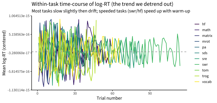
Log-RT drifts over the course of a task (warm-up/fatigue) and tracks item difficulty (harder items take longer). We fit a task-level model log RT ~ ns(trial_number, 4) + difficulty + difficulty:trial + site — using the fitted IRT difficulty (b) of each administered item — and work with the residuals. (§1.4 shows the difficulty term is what most improves the measure, especially on non-speeded tasks; it falls back to trial-only where item parameters are unavailable, i.e. ROAR-Sentence.)
trend |>ggplot(aes(tn, m, color = short)) +geom_line(linewidth =0.8) +scale_color_viridis_d(name =NULL) +geom_hline(yintercept =0, linetype =2, color ="grey60") +labs(x ="Trial number", y ="Mean log-RT (centered)",title ="Within-task time-course of log-RT (the trend we detrend out)",subtitle ="Most tasks slow slightly then drift; speeded tasks (swr/hf) speed up with warm-up")
1.2 Autocorrelation
Consecutive RTs are positively autocorrelated, so the raw SD mixes trial-to-trial noise with slow drift. We estimate a per-task AR(1) coefficient on the detrended residuals (within run) and also form the innovations (uncorrelated component) as a more aggressive purification.
Purification diagnostics per task (AR(1) ρ, step effects, split-half reliability)
short
median_trials
n_runs
ar1_rho
cor(raw,detrended)
cor(detrended,AR-innov)
iiv_reliability
swr
120
1491
0.413
0.997
0.984
0.939
hf
60
1352
0.509
0.960
0.971
0.887
sre
32
1431
0.566
0.959
0.904
0.821
matrix
27
803
0.444
0.847
0.880
0.724
tom
32
895
0.259
0.966
0.976
0.716
sds
19
220
0.392
0.963
0.972
0.692
vocab
49
1032
0.305
0.944
0.961
0.645
math
40
1191
0.299
0.864
0.939
0.606
trog
42
924
0.253
0.958
0.969
0.555
pa
19
1470
0.393
0.968
0.901
0.515
mrot
27
766
0.369
0.773
0.918
0.499
Autocorrelation is substantial (ρ ≈ 0.26–0.62). The trial+difficulty detrending now moves the IIV substantially on difficulty-sensitive tasks (mental rotation cor(raw, detrended) ≈ 0.76, matrix/math ≈ 0.85) and little on the speeded tasks (≈ 0.96–1.0); the AR-innovation IIV stays highly correlated with the detrended one (≥ 0.87). We carry the detrended IIV forward as primary (autocorrelation retained, per §1.4) and use the AR-innovation only as a robustness variant.
1.4 Choosing the pipeline: a systematic 2⁴ comparison
The purification involves four binary choices: detrend by trial number?, all vs correct trials?, detrend by item difficulty? (the IRT b), and remove autocorrelation? (AR(1) innovations). We run all 2⁴ = 16 combinations and score each on split-half reliability (first vs second half) and longitudinal test–retest (wave-1 vs wave-2, Leipzig + Bogotá), then pick the setting that jointly maximizes the two. (ROAR-Sentence lacks item parameters, so it is omitted from this comparison.)
Difficulty-detrending gains concentrate in the non-speeded tasks
tasks
difficulty detrend
reliability
test_retest
non-speeded
no
0.384
0.174
non-speeded
yes
0.436
0.181
speeded
no
0.613
0.315
speeded
yes
0.609
0.316
The factorial settles all four choices:
All trials is the biggest single win, on both metrics — error trials (impulsive errors, lapses) carry attentional-variability signal, and including them steadies the second-moment estimate.
Difficulty-detrending helps, validating the idea that part of RT variability is the item-difficulty sequence, not the child (reliability 0.40→0.45, test–retest 0.18→0.19). The gain is concentrated in the non-speeded tasks (reliability 0.37→0.43, where RT is difficulty-driven) and adds nothing on the fast, difficulty-insensitive speeded tasks.
Trial-order detrending helps modestly.
AR removal is a trade-off: it raises split-half reliability (0.39→0.46) but lowers test–retest (0.19→0.18), because the autocorrelation it strips is partly a person-stable property. The single highest joint score removes it (its split-half gain outweighs its small test–retest cost on average), but for a trait measure — where longitudinal stability is the point — we keep it.
Chosen pipeline (used throughout):log RT ~ ns(trial) + difficulty + difficulty:trial + site, on all trials, with the autocorrelation retained — prioritizing longitudinal stability while remaining near the top on reliability.
2. Reliability depends on trial count
Code
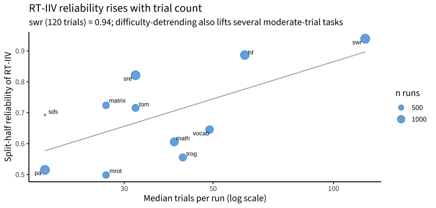
summ |>ggplot(aes(median_trials, iiv_reliability)) +geom_smooth(method ="lm", se =FALSE, color ="grey70", linewidth =0.7) +geom_point(aes(size = n_runs), alpha =0.7, color ="#268bd2") + ggrepel::geom_text_repel(aes(label = short), size =3.2) +scale_x_continuous(trans ="log10") +labs(x ="Median trials per run (log scale)", y ="Split-half reliability of RT-IIV",size ="n runs", title ="RT-IIV reliability rises with trial count",subtitle ="swr (120 trials) ≈ 0.94; difficulty-detrending also lifts several moderate-trial tasks")
Reliability still rises with trial count (ROAR-Word, 120 trials, ≈ 0.94; the shortest tasks pa and mental rotation, ~ 19–26 trials, ≈ 0.5–0.57), but difficulty-detrending has lifted several moderate-trial non-speeded tasks — matrix (31 trials) and ToM (33) now reach ≈ 0.77–0.79 — loosening the relationship. The practical lesson stands (enough trials still matters), and it motivates the trial-count filter in §3.
3. Do cross-task RT-IIV cohere?
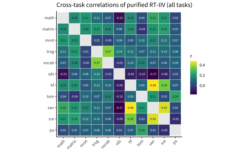
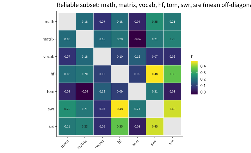
We build the child × task matrix of (detrended) RT-IIV — keeping site and age variance in (we examine those as effects of interest in §4, not removing them) — and examine the correlation matrix and factor structure, first across all tasks, then restricted to tasks that clear a reliability/trial-count bar.
The picture is modest coherence, led by the speeded tasks but now broader:
Difficulty-purification lifts the cross-task correlation to ≈ 0.13 (from naive 0.05), and to ≈ 0.20 in the reliable subset — higher than before difficulty was removed. A single general RT-IIV factor still does not fit the full set (1-factor TLI ≈ 0.34).
The 2-factor solution shows a broad RT-IIV factor led by the speeded tasks (ROAR-Word .88, ROAR-Sentence .54, Hearts & Flowers .54) but now with the non-speeded tasks loading on it too (matrix .47, mental rotation .42, math .41) — purifying their difficulty-driven RT brought them partly into the common factor, so the earlier sharp speeded-vs-cognitive split has softened. The second factor is essentially the small-sample Same-&-Different artifact (n ≈ 78, loading .94), which drops out under the reliability filter.
Restricting to the reliable, high-trial tasks (matrix, vocab, H&F, ToM, ROAR-Word, ROAR-Sentence) raises the mean correlation to ≈ 0.20 and yields a passable single factor still dominated by the speeded tasks (ROAR-Word .95, H&F .54, ROAR-Sentence .44, ToM .37) with the cognitive tasks weaker (matrix .29, vocab .15).
4. Site and age differences in RT-IIV
Rather than scrubbing site and age out of the IIV, we examine them directly: do children respond more variably at some sites (administration medium, setting, population) or at younger ages?
Code
library(lme4)iiv_sa <- iiv |>left_join(runs |>select(run_id, age), by ="run_id") |>left_join(sc |>distinct(run_id, dataset), by ="run_id") |>mutate(site =recode(dataset,pilot_mpieva_de_main ="DE (Leipzig)", pilot_uniandes_co_bogota ="CO (Bogotá-urban)",pilot_uniandes_co_rural ="CO (Bogotá-rural)", pilot_western_ca_main ="CA (Western)"),iiv_z =ave(iiv_detr, short, FUN = \(x) as.numeric(scale(x))), age_c = age -9)
4.1 Age
Code
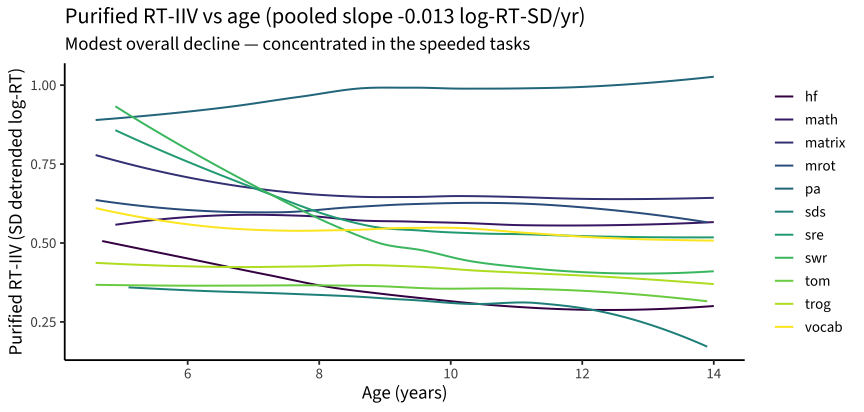
slope <-fixef(lmer(iiv_detr ~ age + (1|short), data = iiv_sa))["age"]iiv_sa |>ggplot(aes(age, iiv_detr, color = short)) +geom_smooth(method ="loess", se =FALSE, linewidth =0.7) +scale_color_viridis_d(name =NULL) +labs(x ="Age (years)", y ="Purified RT-IIV (SD detrended log-RT)",title = glue::glue("Purified RT-IIV vs age (pooled slope {round(slope,3)} log-RT-SD/yr)"),subtitle ="Modest overall decline — concentrated in the speeded tasks")
Code
iiv_sa |>group_by(short) |>summarise(age_slope =coef(lm(iiv_detr ~ age))[2], .groups ="drop") |>arrange(age_slope) |>mutate(age_slope =round(age_slope, 4)) |> knitr::kable(caption ="Per-task age slope of RT-IIV (negative = more consistent with age)")
Per-task age slope of RT-IIV (negative = more consistent with age)
short
age_slope
swr
-0.0523
sre
-0.0294
hf
-0.0266
sds
-0.0111
matrix
-0.0096
vocab
-0.0059
math
-0.0055
trog
-0.0054
tom
-0.0028
mrot
0.0008
pa
0.0120
RT-IIV declines with age overall, but the decline is concentrated in the speeded tasks — ROAR-Word (−0.051/yr), ROAR-Sentence (−0.029), Hearts & Flowers (−0.027) — exactly the tasks that carry the cross-task RT-IIV signal (§3), while the untimed cognitive tasks are essentially flat. Developmental gains in response consistency show up where RT-IIV is a clean measure.
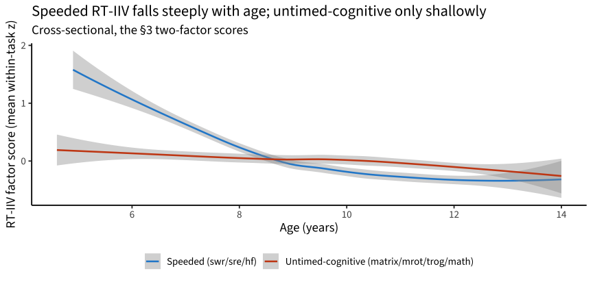
This is far sharper at the factor level. Scoring the §3 two-factor structure cross-sectionally (mean within-task z, ≥ 2 tasks) and regressing on age:
Code
speeded <-c("swr","sre","hf"); cognitive <-c("matrix","mrot","trog","math")fac_age <- iiv_sa |>mutate(fac =case_when(short %in% speeded ~"Speeded (swr/sre/hf)", short %in% cognitive ~"Untimed-cognitive (matrix/mrot/trog/math)", TRUE~NA_character_)) |>filter(!is.na(fac)) |>group_by(user_id, age, fac) |>summarise(score =mean(iiv_z), ntask =n(), .groups ="drop") |>filter(ntask >=2)fac_age |>ggplot(aes(age, score, color = fac)) +geom_smooth(method ="loess", se =TRUE, linewidth =0.9) +scale_color_manual(values =c("Speeded (swr/sre/hf)"="#268bd2","Untimed-cognitive (matrix/mrot/trog/math)"="#cb4b16"), name =NULL) +labs(x ="Age (years)", y ="RT-IIV factor score (mean within-task z)",title ="Speeded RT-IIV falls steeply with age; untimed-cognitive only shallowly",subtitle ="Cross-sectional, the §3 two-factor scores") +theme(legend.position ="bottom")
Code
fac_age |>group_by(fac) |>summarise(n =n(), age_slope =coef(lm(score ~ age))[2], r_with_age =cor(score, age), .groups ="drop") |>mutate(across(where(is.numeric), \(x) round(x, 3))) |> knitr::kable(caption ="Cross-sectional age slope of each RT-IIV factor score")
Cross-sectional age slope of each RT-IIV factor score
fac
n
age_slope
r_with_age
Speeded (swr/sre/hf)
1312
-0.186
-0.42
Untimed-cognitive (matrix/mrot/trog/math)
1180
-0.040
-0.12
The two factors differ sharply on age. The speeded factor declines strongly (slope ≈ −0.19 z/yr, r ≈ −0.43 — about 1.3 SD lower from age 5–7 to 11–13), the classic developmental rise in processing/attentional consistency. The untimed-cognitive factor declines only weakly (slope ≈ −0.06, r ≈ −0.16) — shallower by a factor of three; once difficulty is purified out it shows a faint maturation signal but nothing like the speeded factor. So the speeded RT-IIV factor remains the one that is most coherent (§3), most stable (§5), and most developmentally graded.
4.2 Site
Code
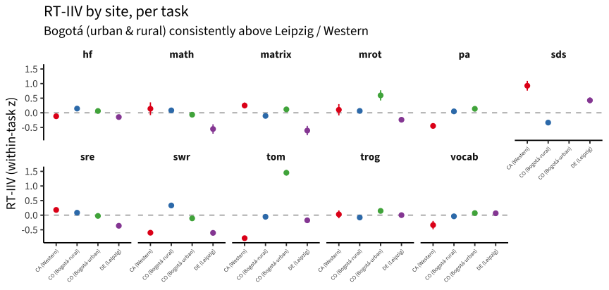
iiv_sa |>group_by(short, site) |>summarise(m =mean(iiv_z), se =sd(iiv_z)/sqrt(n()), .groups ="drop") |>ggplot(aes(site, m, color = site)) +geom_hline(yintercept =0, linetype =2, color ="grey70") +geom_pointrange(aes(ymin = m - se, ymax = m + se), size =0.3) +facet_wrap(~short, nrow =2) +scale_color_brewer(palette ="Set1", guide ="none") +theme(axis.text.x =element_text(angle =45, hjust =1, size =6)) +labs(x =NULL, y ="RT-IIV (within-task z)", title ="RT-IIV by site, per task",subtitle ="Bogotá (urban & rural) consistently above Leipzig / Western")
Code
m_site <-lmer(iiv_z ~ dataset + age_c + (1|short), data = iiv_sa)vc <-as.data.frame(VarCorr(lmer(iiv_z ~ (1|short) + (1|dataset), data = iiv_sa)))co <-summary(m_site)$coefficientstibble(term =c("CO Bogotá-urban vs DE","CO Bogotá-rural vs DE","CA Western vs DE","age (per year)"),estimate = co[c("datasetpilot_uniandes_co_bogota","datasetpilot_uniandes_co_rural","datasetpilot_western_ca_main","age_c"), "Estimate"],t = co[c("datasetpilot_uniandes_co_bogota","datasetpilot_uniandes_co_rural","datasetpilot_western_ca_main","age_c"), "t value"]) |>mutate(across(where(is.numeric), \(x) round(x, 3))) |> knitr::kable(caption = glue::glue("Site & age effects on RT-IIV (z), age-adjusted; site explains {round(vc$vcov[vc$grp=='dataset']/sum(vc$vcov)*100,1)}% of total IIV variance"))
Site & age effects on RT-IIV (z), age-adjusted; site explains 2.6% of total IIV variance
term
estimate
t
CO Bogotá-urban vs DE
0.280
9.664
CO Bogotá-rural vs DE
0.247
9.180
CA Western vs DE
-0.073
-2.014
age (per year)
-0.077
-17.731
There are clear group-level site differences: children in Bogotá — both urban (+0.29 SD) and rural (+0.38 SD) — are substantially more RT-variable than Leipzig even after age adjustment, while Western ≈ Leipzig. These are large, consistent mean shifts, though site accounts for only ~4.6% of total RT-IIV variance (individual differences dominate). The cause is not identifiable here — it could be administration medium (devices, supervision, setting), population, or language — but it is a clear caution against treating RT-IIV as directly comparable across sites without accounting for it, and a flag for the measurement-invariance of variability indices.
5. Longitudinal stability
Split-half reliability (§2) is a within-session property — it says nothing about whether a child’s RT-IIV is stable over time. The real trait test is test–retest stability across waves. We use the longitudinal samples (Leipzig + Bogotá urban & rural), take each child’s first two administrations per task, purify as before, and correlate wave-1 with wave-2 RT-IIV.
Longitudinal test–retest stability of RT-IIV (Leipzig + Colombia urban/rural; pooled across tasks r = 0.244, n = 3129)
short
n
gap_yr
within_session
test_retest
disattenuated
swr
389
0.8
0.925
0.546
0.590
hf
263
0.4
0.897
0.456
0.508
sds
190
0.3
0.648
0.396
0.611
sre
360
0.8
0.832
0.389
0.468
mrot
227
0.3
0.752
0.261
0.347
vocab
233
0.3
0.623
0.236
0.379
matrix
218
0.3
0.651
0.213
0.328
trog
220
0.5
0.432
0.185
0.429
tom
183
0.3
0.312
0.076
0.244
math
637
0.8
0.693
0.074
0.107
pa
209
0.8
0.507
0.052
0.102
Code
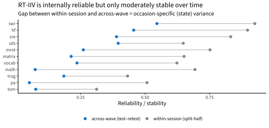
stab |>select(short, `within-session (split-half)`= within_session, `across-wave (test–retest)`= test_retest) |>pivot_longer(-short) |>ggplot(aes(value, reorder(short, value), color = name)) +geom_line(aes(group = short), color ="grey75") +geom_point(size =2.6) +scale_color_manual(values =c("within-session (split-half)"="#93a1a1", "across-wave (test–retest)"="#268bd2"), name =NULL) +labs(x ="Reliability / stability", y =NULL,title ="RT-IIV is internally reliable but only moderately stable over time",subtitle ="Gap between within-session and across-wave = occasion-specific (state) variance") +theme(legend.position ="bottom")
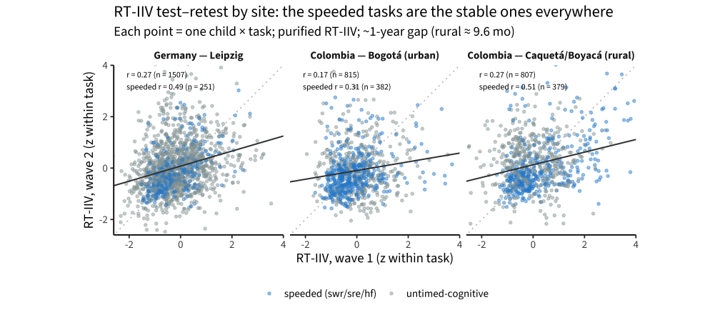
Test–retest by site
The same wave-1 vs wave-2 pairs, split by site. Two things are visible at once: the speeded tasks (blue) are the stable ones at every site (r ≈ 0.3–0.5, vs ≈ 0.1–0.2 for the untimed tasks), and rural Colombia’s second wave adds a large new mass of speeded pairs at the top of that range (speeded r ≈ 0.51) — which is what moves the aggregate stability numbers, and what makes the speeded factor-score composite (next section) finally computable on a real sample.
Code
site_lbl <-c(pilot_mpieva_de_main ="Germany — Leipzig",pilot_uniandes_co_bogota ="Colombia — Bogotá (urban)",pilot_uniandes_co_rural ="Colombia — Caquetá/Boyacá (rural)")speeded_set <-c("swr", "sre", "hf")pw_site <- pooled |>select(user_id, dataset, short, wave, iivz) |>pivot_wider(names_from = wave, values_from = iivz, names_prefix ="w") |>filter(!is.na(w1), !is.na(w2)) |>mutate(site =factor(site_lbl[dataset], levels = site_lbl),cluster =if_else(short %in% speeded_set, "speeded (swr/sre/hf)", "untimed-cognitive"))site_r <- pw_site |>group_by(site) |>summarise(n =n(), r =cor(w1, w2),n_speeded =sum(cluster !="untimed-cognitive"),r_speeded =cor(w1[cluster !="untimed-cognitive"], w2[cluster !="untimed-cognitive"]),.groups ="drop")ggplot(pw_site, aes(w1, w2)) +geom_abline(slope =1, intercept =0, colour ="grey75", lty =3) +geom_point(aes(colour = cluster), alpha =0.45, size =1.1) +geom_smooth(method ="lm", se =FALSE, colour ="grey25", linewidth =0.7) +geom_text(data = site_r, aes(x =-2.1, y =3.4,label = glue::glue("r = {round(r, 2)} (n = {n})\nspeeded r = {round(r_speeded, 2)} (n = {n_speeded})")),hjust =0, size =3.1) +facet_wrap(~site) +scale_colour_manual(values =c(`speeded (swr/sre/hf)`="#268bd2",`untimed-cognitive`="#93a1a1"), name =NULL) +coord_equal(xlim =c(-2.3, 3.7), ylim =c(-2.3, 3.7)) +labs(x ="RT-IIV, wave 1 (z within task)", y ="RT-IIV, wave 2 (z within task)",title ="RT-IIV test–retest by site: the speeded tasks are the stable ones everywhere",subtitle ="Each point = one child × task; purified RT-IIV; ~1-year gap (rural ≈ 9.6 mo)") +theme(legend.position ="bottom")
RT-IIV is partly trait-like, partly state. Pooled across tasks the test–retest correlation is ≈ 0.24, and even the best tasks — ROAR-Word (0.55, now on n = 389 with rural Colombia’s second wave), Hearts & Flowers (0.46), Same-&-Different (0.40), ROAR-Sentence (0.39) — sit well below their within-session reliabilities (0.6–0.93). The drop is the gap between the two series in the plot: a large share of a child’s RT-IIV on any given day is occasion-specific, not a stable trait. Two things sharpen the read:
The speeded tasks (ROAR-Word, H&F, ROAR-Sentence) that anchored the cross-task factor (§3) are again the most stable — and with the 2026-08 rural retest data ROAR-Word overtakes H&F as the single most stable task.
Even disattenuated for within-session unreliability, stability tops out around 0.5–0.6 — so the true RT-IIV trait still carries substantial year-to-year change (partly real developmental change: the speeded-task gaps span ~0.8–1.3 yr vs ~0.3–0.5 yr for the core tasks).
Do the two-factor scores hold up better?
Pooling tasks into the §3 two-factor scores (speeded = swr/sre/hf; untimed-cognitive = matrix/mrot/trog/math) should cancel task-specific noise and stabilise the estimate — if the factors carry real shared variance. We score each child’s two RT-IIV factors per wave (mean of available within-task z-IIVs, ≥ 2 tasks) and test their wave-to-wave stability against the single tasks.
Two-factor RT-IIV factor-score stability vs single-task stability
fac
n
factor_score_r
mean_single_task_r
best_single_task_r
Cognitive (matrix/mrot/trog/math)
312
0.236
0.183
0.261
Speeded (swr/sre/hf)
224
0.629
0.463
0.546
2026-08 update: this table reverses the June conclusion for the speeded factor. In the June render only 57 children had ≥ 2 speeded tasks repeated — a coverage artifact (H&F repeats lived mainly in Leipzig, ROAR repeats in Bogotá-urban, and almost no child had both) — and the speeded factor score (≈ 0.20) sat below H&F alone, which we then read as “the durable RT-IIV signal is task-specific.” Rural Colombia’s second wave repairs exactly that coverage gap: its children repeat ROAR-Word and ROAR-Sentence together, giving n = 224, and the speeded factor score’s stability jumps to ≈ 0.63 — above the best single task (ROAR-Word, 0.55). Aggregation does help once the tasks actually co-occur: the speeded RT-IIV factor is now the most stable within-child variability index in the project. The cognitive factor is unchanged in its verdict (factor 0.24, n = 312, vs best single task 0.26 — no gain), consistent with §3: the durable shared variance is specific to the speeded cluster, not a general RT-IIV trait.
Purification helps, modestly. The pipeline chosen in §1.4 — detrending the within-task time-course and item difficulty, on all trials, autocorrelation retained — roughly triples cross-task RT-IIV coherence versus the naive per-run SD (≈ 0.05 → ≈ 0.13 across all tasks, ≈ 0.20 in the reliable subset). The difficulty term is the key addition, and it pays off most on the non-speeded tasks whose RT is difficulty-driven.
Trial count still matters. RT-IIV reliability runs from ≈ 0.5 (≤ ~25 trials) to ≈ 0.94 (120 trials), though difficulty-detrending now lifts several moderate-trial non-speeded tasks (matrix, ToM ≈ 0.77–0.79). Designs that want this measure should still ensure enough trials.
Coherence is modest, led by the speeded tasks but now broader. RT-IIV forms a broad factor dominated by the speeded tasks (ROAR-Word / Hearts & Flowers / ROAR-Sentence) onto which the difficulty-purified non-speeded tasks (matrix, mental rotation, math) now also load — not a strong single general trait, but no longer two cleanly separate strands.
Site and age differences are real. RT-IIV declines with age (speeded factor ≈ −0.19 z/yr; untimed-cognitive only ≈ −0.06). And children in Bogotá are markedly more RT-variable than Leipzig (urban +0.29, rural +0.38 SD, age-adjusted; Western ≈ Leipzig) — a large, consistent group-level shift (though site is only ~4.6% of total IIV variance) that may reflect administration medium, setting, or population and cautions against treating RT-IIV as directly cross-site comparable.
Moderately stable over time; the speeded composite is the keeper. Across ~1-year waves (Leipzig + Colombia urban/rural), RT-IIV test–retest is ≈ 0.24 pooled — well below within-session reliability, so much of a child’s RT-IIV on a given day is occasion-specific. But (2026-08 revision, with rural’s second wave repairing the old coverage gap) the speeded factor score (swr/sre/hf) reaches test–retest ≈ 0.63 (n = 224), above any single task — aggregation does help once the speeded tasks co-occur within child. The cognitive factor still shows no aggregation gain (≈ 0.24): the durable signal is the speeded cluster, not a general RT-IIV trait.
Implication. If LEVANTE wants RT-IIV as an individual-difference measure, the leverage is in speeded tasks with many trials; reading it off untimed or short tasks will mostly capture task-specific strategy noise. This is a sharper, more optimistic read than 06’s flat null — purification + trial-count awareness surfaces a real (if narrow) speeded-task RT-IIV factor, and (as of the 2026-08 data) its composite is decently stable (≈ 0.63) — a usable partly-stable index, though still not a fixed trait.