Sentence Understanding (TROG) — does character skin tone function differently across samples?
ImportantAI-generated — not for publication
The code and prose in this chapter were written by Claude Code (an AI coding agent) under human direction. They have not been line-by-line verified by a human and must not be published or cited as-is.
WarningPreliminary & unvetted analysis
These are exploratory analyses of preliminary, in-progress LEVANTE data. Results have not been reviewed or validated and require checking by the LEVANTE Data Coordinating Center before any use.
Question
The TROG pictures show many children and adults, drawn with a range of skin tones. If children respond differently to characters who do or don’t look like them, an item’s difficulty could depend on the skin tone of the people it depicts, and could depend on it differently in different samples (e.g. rural vs urban Colombia, Colombia vs Germany). That would be differential item functioning (DIF) tied to stimulus skin tone, and it would mean the art costs some children points.
This chapter (1) measures the skin tone of every person drawn in the TROG art and (2) asks whether item skin tone predicts group differences in accuracy (item DIF) or which picture children choose.
What “match” can and cannot mean here. LEVANTE collects no child-level race, ethnicity or skin-tone data (none in participants or surveys). A match/mismatch predictor can therefore only be defined at the sample level: we ask whether a sample as a whole is relatively better or worse on items depicting darker- or lighter-skinned characters than a reference sample. Whether a given direction is a “match” depends on the skin-tone composition of each sample, which the site teams know and we do not. The tests below are two-sided for that reason.
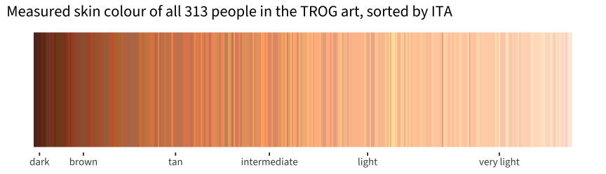
Method (details and code in tasks/trog_skin_tone/README.md). Images are the production set (levante-assets-prod/visual/trog/, cached 2026-09-04). People were found with a COCO Mask R-CNN detector, and each person’s face was segmented with a human-parsing model (SegFormer, ATR labels). Skin colour is the median CIELAB colour of the dominant face-pixel cluster, which drops eyes, mouth and blush. It is summarised as the Individual Typology Angle (ITA = atan((L* − 50)/b*); higher = lighter). Every measurement was checked by eye on contact sheets: 35 animal/object “faces” (horses, dogs, monkeys, turtles…) were removed, 6 people seen from behind were measured on arms/legs, and duplicate readings were merged. ITA bands come from dermatology photographs, so here they are descriptive labels for stylised art, not claims about the characters’ ethnicity.
Code
bands <-tibble(lo =c(-Inf, -30, 10, 28, 41, 55), hi =c(-30, 10, 28, 41, 55, Inf),band =c("dark", "brown", "tan", "intermediate", "light", "very light"))people <- people |>mutate(hex =rgb(r, g, bl, maxColorValue =255),band =cut(ITA, c(-Inf, -30, 10, 28, 41, 55, Inf), labels = bands$band)) |>arrange(ITA) |>mutate(rank =row_number())ggplot(people, aes(x = rank, y =1, fill = hex)) +geom_tile(height =1) +scale_fill_identity() +scale_x_continuous(breaks = people |>group_by(band) |>summarise(m =median(rank)) |>pull(m),labels =levels(people$band)) +labs(x =NULL, y =NULL,title =glue("Measured skin colour of all {nrow(people)} people in the TROG art, sorted by ITA")) +theme(axis.text.y =element_blank(), axis.ticks.y =element_blank(), axis.line =element_blank())
Code
people |>count(band) |>mutate(share = scales::percent(n /sum(n), 1)) |> knitr::kable(col.names =c("ITA band", "People", "Share"),caption =glue("{nrow(people)} people in {n_distinct(people$image)} of {nrow(imgs)} images"))
313 people in 229 of 442 images
ITA band
People
Share
dark
7
2%
brown
44
14%
tan
63
20%
intermediate
46
15%
light
68
22%
very light
85
27%
The art is fairly diverse: about one character in six falls in the brown/dark bands and one in five in the tan band. Items 81–103 (added after Bishop’s original set) are, if anything, slightly darker on average than items 1–80.
Code
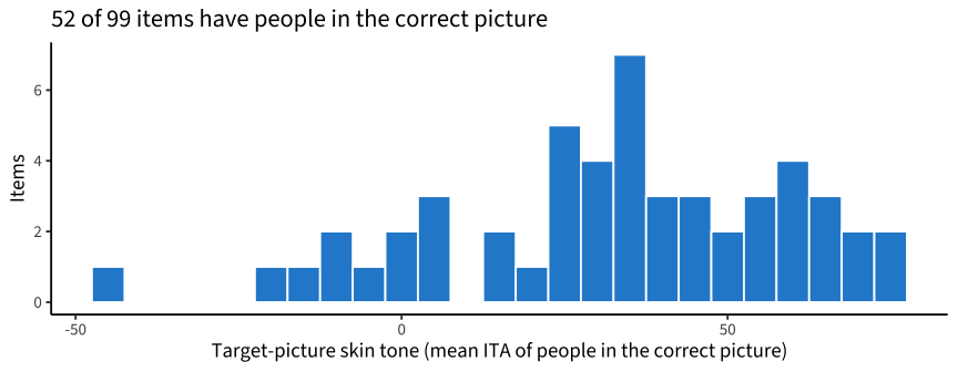
res$item_feat |>filter(!is.na(target_ita)) |>ggplot(aes(x = target_ita)) +geom_histogram(binwidth =5, fill ="#268bd2", color ="white") +labs(x ="Target-picture skin tone (mean ITA of people in the correct picture)", y ="Items",title =glue("{sum(!is.na(res$item_feat$target_ita))} of 99 items have people in the correct picture"))
2. Data
Each child’s first TROG run (cross-sectional), 2026-08-24 trials snapshot. Items are mapped to pictures with the corpus (trog-item-bank.csv). The mapping agrees with children’s recorded responses, and corpus-keyed correctness matches the released correct field.
Code
res$id_check |>left_join(res$n_runs, by ="grp") |>transmute(Sample = grp, Children = n.y, Trials = n.x,`Response in item's picture set`= scales::percent(in_set, .1),`Corpus key = recorded correct`= scales::percent(agree, .1)) |> knitr::kable()
Sample
Children
Trials
Response in item’s picture set
Corpus key = recorded correct
Bogotá
472
26687
99.3%
99.3%
CO (MPIB intl)
81
2664
100.0%
100.0%
Leipzig
275
19135
99.5%
99.5%
Rural CO
522
23875
99.9%
99.9%
Western CA
226
9957
99.9%
99.9%
Bogotá is the reference sample throughout. Rural CO vs Bogotá is the cleanest contrast: same Spanish translation, same audio, same age range, so the pictures’ content is the main thing that differs in how items are experienced. Leipzig (German) and Western Canada (English) contrasts also carry translation differences. CO (MPIB intl) is a smaller es-CO sample of much younger children (4.5–8.4 years). Leipzig is the only German TROG sample, so no urban/rural split is possible within Germany yet.
3. Does target skin tone predict item DIF?
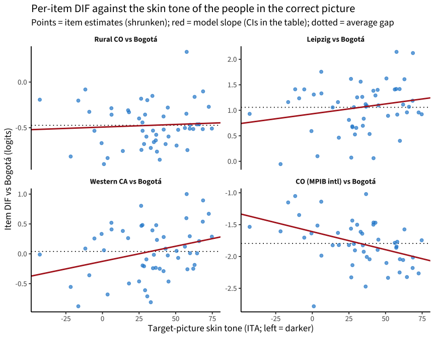
Explanatory item-response model (Rasch with LEVANTE’s fixed 4AFC guessing floor): correct ~ group × target skin tone + (1 | child) + (1 + group | item), fit to the items whose correct picture shows people. The group × skin tone term is the test. It is per 10° of ITA, in logits. Because each item has its own random group effect, the test asks whether skin tone explains item-level DIF beyond ordinary item-to-item DIF.
Code
res$dif_tab |>filter(term %in%c("g", "g:ita10")) |>select(contrast, n_runs, n_items, term, est, se, p, sd_item_dif) |>pivot_wider(names_from = term, values_from =c(est, se, p)) |>transmute(Contrast =paste(contrast, "vs Bogotá"), Children = n_runs, Items = n_items,`Overall gap (logits)`=sprintf("%.2f", est_g),`Skin tone × group, per 10° ITA [95% CI]`=ci(`est_g:ita10`, `se_g:ita10`),p =sprintf("%.2f", `p_g:ita10`),`Item DIF SD`=sprintf("%.2f", sd_item_dif)) |> knitr::kable(align ="lrrrrrr")
Contrast
Children
Items
Overall gap (logits)
Skin tone × group, per 10° ITA [95% CI]
p
Item DIF SD
Rural CO vs Bogotá
990
52
-0.47
0.006 [-0.046, 0.058]
0.83
0.35
Leipzig vs Bogotá
743
52
1.06
0.039 [-0.044, 0.122]
0.36
0.62
Western CA vs Bogotá
694
52
0.04
0.051 [-0.031, 0.132]
0.22
0.59
CO (MPIB intl) vs Bogotá
549
50
-1.80
-0.057 [-0.140, 0.027]
0.18
0.49
Code
lv <-paste(c("Rural CO", "Leipzig", "Western CA", "CO (MPIB intl)"), "vs Bogotá")fx <- res$dif_tab |>select(contrast, term, est) |>pivot_wider(names_from = term, values_from = est) |>mutate(contrast =factor(paste(contrast, "vs Bogotá"), levels = lv))res$item_dif |>mutate(contrast =factor(paste(contrast, "vs Bogotá"), levels = lv)) |>ggplot(aes(x = target_ita, y = dif)) +geom_hline(data = fx, aes(yintercept = g), lty =3) +geom_point(alpha = .7, color ="#268bd2") +geom_abline(data = fx, aes(intercept = g -`g:ita10`* res$ita_ref /10, slope =`g:ita10`/10),color ="firebrick", linewidth =1) +facet_wrap(~contrast, scales ="free_y") +labs(x ="Target-picture skin tone (ITA; left = darker)", y ="Item DIF vs Bogotá (logits)",title ="Per-item DIF against the skin tone of the people in the correct picture",subtitle ="Points = item estimates (shrunken); red = model slope (CIs in the table); dotted = average gap")
4. Are children drawn to pictures by skin tone?
The accuracy test uses only the correct picture. Children’s choices carry more information: on 55 items, at least two of the four pictures show people, and these usually differ in skin tone. A conditional logit over the pictures on screen, with a fixed effect for every picture (each picture’s overall pull, shared across samples), estimates whether a sample is more or less drawn to pictures of darker vs lighter characters than Bogotá children are. It also includes a sample-specific pull toward the correct picture, so accuracy differences can’t leak into the skin-tone term. Negative = relatively more drawn to darker-skinned characters. Standard errors are clustered by item. The errors-only model keeps only trials where the child chose a wrong picture and asks which distractor they picked.
43791 trials on 55 items; errors-only: 6851 trials
Model
Sample
Skin-tone pull vs Bogotá, per 10° ITA [95% CI]
p
all trials
Rural CO
-0.017 [-0.039, 0.004]
0.117
all trials
Leipzig
-0.025 [-0.092, 0.041]
0.457
all trials
Western CA
0.003 [-0.028, 0.033]
0.859
all trials
CO (MPIB intl)
-0.063 [-0.101, -0.026]
0.001
errors only
Rural CO
-0.012 [-0.046, 0.022]
0.497
errors only
Leipzig
-0.134 [-0.331, 0.063]
0.182
errors only
Western CA
0.026 [-0.048, 0.099]
0.497
errors only
CO (MPIB intl)
-0.054 [-0.113, 0.005]
0.074
Is the MPIB-intl signal about the sample or about age?
The MPIB-intl children are much younger than the Bogotá children, so the choice model is refit on children aged 4.5–8.4 in every sample. The table also shows whether the skin-tone pull changes with age within Bogotá + rural, and the item-DIF model on the age-matched subset. That last fit gave an lme4 convergence warning (its overall-gap term is unreliable), but its skin-tone term agrees with the full-sample fit in §3.
Age-matched n: Bogotá = 130, CO (MPIB intl) = 80, Rural CO = 216
Model
Term
Estimate [95% CI]
p
all trials, ages 4.5-8.4
skin × rural
-0.035 [-0.070, 0.000]
0.050
all trials, ages 4.5-8.4
skin × MPIB intl
-0.059 [-0.098, -0.020]
0.003
Bogotá + rural, age interaction
skin × age (per year)
0.010 [-0.000, 0.019]
0.057
Bogotá + rural, age interaction
skin × rural
-0.011 [-0.034, 0.011]
0.317
item DIF, MPIB vs Bogotá ages 4.5-8.4
skin × MPIB intl (accuracy)
-0.050 [-0.125, 0.025]
0.189
Verdict
The art is diverse. Of 313 depicted people, about 16% are in the brown/dark ITA bands and 20% tan. 52 items show people in the correct picture, 11 of them dark-skinned (ITA < 10).
Rural vs urban Colombia: no skin-tone DIF. This is the cleanest contrast, with the same translation and audio. Rural children score about 0.47 logits below Bogotá children overall, and that gap does not depend on the target’s skin tone: +0.006 logits per 10° ITA [−0.046, 0.058]. The 11 dark-target items show exactly the average gap. Children’s choices tell the same story: rural children are drawn to darker vs lighter characters about as much as Bogotá children are (−0.017 per 10° [−0.039, 0.004]; errors only −0.012). Among children under 8.5 there is a borderline lean toward darker characters in rural vs Bogotá children (−0.035, p = .05). Controlling for age, it shrinks to −0.011 (p = .32), and it does not show up in accuracy. The accuracy data rule out skin-tone effects larger than about 0.05 logits per 10° of ITA.
Leipzig and Western Canada vs Bogotá: no evidence either. The intervals are wider, and these contrasts also carry translation differences. Germany has only one TROG sample (Leipzig), so there is no urban/rural German comparison yet.
One signal: the CO (MPIB intl) sample. These young es-CO children (4.5–8.4 years, n = 80) are somewhat more drawn to pictures of darker-skinned characters than Bogotá children (−0.063 per 10°, p < .001). The effect holds against Bogotá children of the same ages (−0.059, p = .003). Within Bogotá + rural, younger children lean slightly darker (+0.010 per year, p = .06), but that accounts for only part of the difference. The accuracy counterpart has the same sign but is not significant (−0.057 [−0.14, 0.03]): MPIB children do relatively better on darker-target items and worse on lighter-target ones. Whether this is a “match” effect depends on the sample’s composition, which the site team would know. It is a small sample, and the signal is in choices rather than in accuracy, so it needs replication before it is acted on.
Stories was not analysed: its art is uniformly diverse, and ToM item identities are still being repaired (see the Stories chapter).
Bottom line. In the samples where the question is best posed, stimulus skin tone does not produce performance decrements on Sentence Understanding. The one hint of a skin-tone preference (a young, small Colombian sample) does not yet translate into a reliable accuracy difference.