Math — item calibration & re-scoring diagnostics

AI-generated — not for publication

The code and prose in this chapter were written by Claude Code (an AI coding agent) under human direction. They have not been line-by-line verified by a human and must not be published or cited as-is.

Preliminary & unvetted analysis

These are exploratory analyses of preliminary, in-progress LEVANTE data. Results have not been reviewed or validated and require checking by the LEVANTE Data Coordinating Center before any use.

Purpose

tasks/math.qmd showed that the Bogotá math T1→T2 “regression to the mean” is the CAT routing high-T1 kids onto number-line items they hadn’t been tested on at T1. Two questions remain:

Why does the CAT serve so many line items to high-θ kids? Bank composition? Information-maximization? A bug?
Why does that depress the IRT score? In principle a properly calibrated Rasch model handles asymmetric item provisioning across modes — every kid should land on the same θ scale regardless of which items they saw. So why doesn’t it?

We answer (1) using the item-parameter table from levante_metadata_scoring. We answer (2) by computing per-kid Rasch MLE ability estimates from the items each child actually saw, and comparing those to the pipeline-reported scores.

source(here::here("common.R"))

scores <- read_rds(here::here("data", "scores_all_sites.rds"))
trials <- load_levante_trials(task_ids = "egma-math")
ip     <- load_item_parameters()

ipm <- ip |>
  filter(task_id == "egma-math", subset == "all_items",
         itemtype == "rasch", model_set == "multigroup_site") |>
  mutate(item_group = str_extract(item_uid, "(?<=math_)[^_]+"))

1. Item bank: where do line items sit?

ig_order <- ipm |>
  group_by(item_group) |>
  summarise(med = median(difficulty), .groups = "drop") |>
  arrange(med) |> pull(item_group)

ipm |>
  mutate(item_group = factor(item_group, levels = ig_order)) |>
  ggplot(aes(x = item_group, y = difficulty, color = item_group)) +
  geom_jitter(width = 0.2, alpha = 0.5) +
  geom_boxplot(outlier.shape = NA, alpha = 0.1, color = "black") +
  geom_hline(yintercept = 0, lty = 3, color = "grey50") +
  scale_color_brewer(palette = "Spectral", guide = "none") +
  labs(x = NULL, y = "Item difficulty (β)",
       title = "Math item difficulty by item_group",
       subtitle = "Rasch multigroup_site / scalar invariance calibration") +
  theme(axis.text.x = element_text(angle = 45, hjust = 1))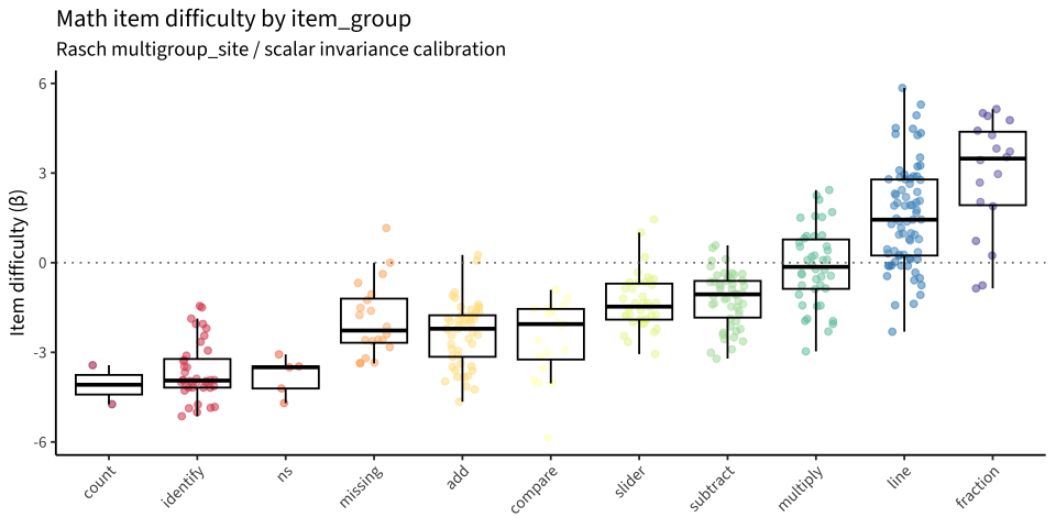

ipm |>
  group_by(item_group) |>
  summarise(
    n_items       = n(),
    median_diff   = median(difficulty),
    p10_diff      = quantile(difficulty, 0.1),
    p90_diff      = quantile(difficulty, 0.9),
    max_diff      = max(difficulty),
    median_n_resp = median(n_responses)
  ) |>
  arrange(median_diff) |>
  knitr::kable(digits = 2)

item_group	n_items	median_diff	p10_diff	p90_diff	max_diff	median_n_resp
count	2	-4.08	-4.61	-3.56	-3.43	87.0
identify	40	-3.95	-4.83	-2.05	-1.45	628.5
ns	5	-3.50	-4.50	-3.23	-3.07	85.0
missing	20	-2.27	-3.35	-0.34	1.16	819.5
add	49	-2.21	-3.83	-1.36	0.26	593.0
compare	20	-2.05	-4.03	-1.41	-0.91	740.0
slider	39	-1.47	-2.24	-0.46	1.45	289.0
subtract	50	-1.06	-2.51	-0.33	0.58	244.5
multiply	42	-0.14	-1.94	1.56	2.43	64.5
line	74	1.44	-0.41	4.05	5.85	83.5
fraction	18	3.49	-0.06	4.94	5.14	19.0

The item bank skews monotonically: counting and identification at β ≈ −4, arithmetic in the middle, line items median β = +1.5, range up to +5.9, and fractions at β ≈ +3. Line items have median ~84 responses each in the calibration sample, vs ~600 for the easy items.

ipm |>
  mutate(diff_bin = cut(difficulty, breaks = c(-Inf, -3, -1, 1, 3, Inf),
                        labels = c("β<-3", "-3 to -1", "-1 to 1",
                                   "1 to 3", "β>3"))) |>
  count(diff_bin, item_group) |>
  ggplot(aes(x = diff_bin, y = n, fill = item_group)) +
  geom_col(position = "stack") +
  scale_fill_brewer(palette = "Spectral") +
  labs(x = "Difficulty band", y = "Items",
       fill = NULL,
       title = "Bank composition by difficulty band",
       subtitle = "Above β=1 the bank is mostly line and fraction items") +
  theme(legend.position = "right")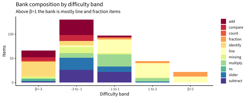

So when the CAT estimates a kid at θ ≈ +1 or higher, the items that maximize Fisher information at that θ are predominantly line items. This is mechanical: max-info items at θ are those with β ≈ θ, and the only items with β > 1 are line/fraction.

2. Join item parameters into the trial data

math_trials <- trials |>
  filter(task_id == "egma-math") |>
  left_join(ipm |> select(item_uid, beta = difficulty,
                          item_group_ip = item_group),
            by = "item_uid")

cat("Math trials with item β attached:",
    sum(!is.na(math_trials$beta)), "/", nrow(math_trials), "\n")

Math trials with item β attached: 183332 / 189370

cat("Distinct items in trials but missing β:",
    n_distinct(math_trials$item_uid[is.na(math_trials$beta)]), "\n")

Distinct items in trials but missing β: 28

math_trials |>
  filter(is.na(beta)) |>
  count(item_uid, name = "n_trials") |>
  arrange(desc(n_trials)) |>
  head(10) |>
  knitr::kable(caption = "Top items in trials but missing from item_parameters")

Top items in trials but missing from item_parameters
item_uid	n_trials
math_compare_10_12	543
math_add_2_2	533
math_ns_identify_2	457
math_identify_3	456
math_count_1	451
math_ns_count_7	451
math_count_4	450
math_ns_count_5	450
math_ns_count_3	449
math_ns_compare_7_4	436

3. Bogotá two-wave sample

math_bog <- scores |>
  filter(dataset == "pilot_uniandes_co_bogota", task_id == "egma-math") |>
  group_by(user_id) |> arrange(age) |>
  mutate(wave = row_number()) |> ungroup() |>
  filter(wave <= 2)

pairs <- math_bog |>
  group_by(user_id) |>
  filter(n_distinct(wave) == 2) |>
  summarise(score_t1 = score[wave == 1], score_t2 = score[wave == 2],
            run_id_t1 = run_id[wave == 1], run_id_t2 = run_id[wave == 2],
            .groups = "drop") |>
  mutate(t1_quartile = ntile(score_t1, 4))

cat("Two-wave Bogotá math kids:", nrow(pairs), "\n")

Two-wave Bogotá math kids: 234

4. For high-T1 kids: did the CAT actually route them to harder items?

twq <- bind_rows(
  math_trials |> filter(dataset == "pilot_uniandes_co_bogota",
                         run_id %in% pairs$run_id_t1) |>
    mutate(wave = "T1") |>
    inner_join(pairs |> select(run_id = run_id_t1, t1_quartile),
               by = "run_id"),
  math_trials |> filter(dataset == "pilot_uniandes_co_bogota",
                         run_id %in% pairs$run_id_t2) |>
    mutate(wave = "T2") |>
    inner_join(pairs |> select(run_id = run_id_t2, t1_quartile),
               by = "run_id")
)

twq |>
  filter(!is.na(beta)) |>
  ggplot(aes(x = factor(t1_quartile), y = beta, fill = wave)) +
  geom_violin(alpha = 0.7, color = NA) +
  geom_boxplot(width = 0.15, position = position_dodge(0.9),
               outlier.shape = NA, alpha = 0.4) +
  scale_fill_manual(values = c(T1 = "#268bd2", T2 = "#d33682")) +
  labs(x = "T1 quartile", y = "Item difficulty β",
       fill = NULL,
       title = "Item difficulty seen by wave × T1 quartile",
       subtitle = "At T2 the CAT routes Q4 (high-T1) kids onto noticeably harder items")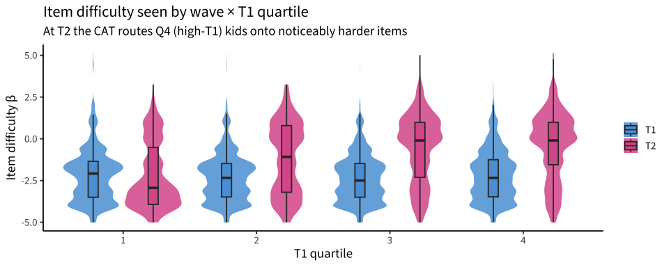

twq |>
  filter(!is.na(beta)) |>
  group_by(t1_quartile, wave) |>
  summarise(median_beta = median(beta),
            mean_beta   = mean(beta),
            n_trials    = n(),
            .groups = "drop") |>
  pivot_wider(names_from = wave, values_from = c(median_beta, mean_beta,
                                                  n_trials)) |>
  knitr::kable(digits = 2)

t1_quartile	median_beta_T1	median_beta_T2	mean_beta_T1	mean_beta_T2	n_trials_T1	n_trials_T2
1	-2.08	-2.94	-2.21	-2.23	4691	2490
2	-2.34	-1.08	-2.31	-1.20	5722	2364
3	-2.50	-0.10	-2.37	-0.56	5463	2370
4	-2.34	-0.10	-2.19	-0.40	6089	2436

5. The critical test: are kids correctly answering the harder items?

For Q4 (high-T1) kids at T2, what’s their accuracy at each β-band? If they’re genuinely at θ ≈ +2 (per T1 score), Rasch predicts ~73% correct on β=+1 items, ~50% on β=+2 items, ~27% on β=+3 items.

rasch_p <- function(theta, beta) 1 / (1 + exp(beta - theta))

q4_t2 <- twq |>
  filter(t1_quartile == 4, wave == "T2", !is.na(beta), !is.na(correct))

# Get each kid's reported T1 θ as their "true" ability for the prediction
q4_t2 <- q4_t2 |>
  inner_join(pairs |> select(user_id, score_t1), by = "user_id")

q4_t2 |>
  mutate(beta_bin = cut(beta, breaks = c(-Inf, -2, -1, 0, 1, 2, Inf))) |>
  group_by(beta_bin) |>
  summarise(
    n_trials   = n(),
    actual_acc = mean(correct, na.rm = TRUE),
    pred_acc   = mean(rasch_p(score_t1, beta), na.rm = TRUE),
    .groups    = "drop"
  ) |>
  pivot_longer(c(actual_acc, pred_acc)) |>
  ggplot(aes(x = beta_bin, y = value, fill = name)) +
  geom_col(position = "dodge") +
  scale_fill_manual(values = c(actual_acc = "#268bd2", pred_acc = "#cb4b16"),
                    labels = c("Observed", "Rasch prediction at T1 θ")) +
  scale_y_continuous(labels = scales::percent) +
  labs(x = "Item difficulty β at T2", y = "P(correct)",
       fill = NULL,
       title = "Q4 (high-T1) kids: observed vs predicted accuracy at T2",
       subtitle = "Prediction uses each kid's T1 θ as 'true' ability")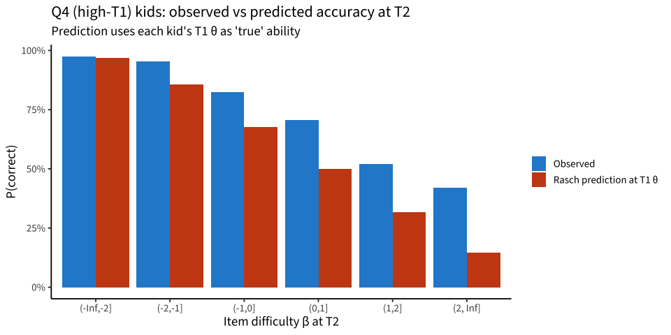

q4_t2 |>
  group_by(item_group_ip) |>
  filter(n() >= 30) |>
  summarise(
    n_trials   = n(),
    median_beta = median(beta),
    actual_acc = mean(correct, na.rm = TRUE),
    pred_acc   = mean(rasch_p(score_t1, beta), na.rm = TRUE),
    .groups    = "drop"
  ) |>
  mutate(gap = actual_acc - pred_acc) |>
  arrange(gap) |>
  knitr::kable(digits = 3,
               caption = "Q4 kids at T2: observed - predicted accuracy by item_group")

Q4 kids at T2: observed - predicted accuracy by item_group
item_group_ip	n_trials	median_beta	actual_acc	pred_acc	gap
identify	290	-3.96	0.986	0.984	0.002
subtract	67	-0.88	0.821	0.782	0.039
compare	124	-2.94	0.976	0.925	0.051
add	33	-1.51	0.909	0.853	0.056
missing	168	-2.57	0.935	0.863	0.071
multiply	99	-0.86	0.869	0.768	0.101
line	1620	0.79	0.686	0.496	0.190
fraction	35	4.42	0.371	0.174	0.198

6. Same diagnostic for ALL quartiles, not just Q4

twq |>
  filter(wave == "T2", !is.na(beta), !is.na(correct)) |>
  inner_join(pairs |> select(user_id, score_t1), by = "user_id") |>
  mutate(beta_bin = cut(beta, breaks = c(-Inf, -2, -1, 0, 1, 2, Inf))) |>
  group_by(t1_quartile, beta_bin) |>
  filter(n() >= 20) |>
  summarise(
    actual_acc = mean(correct, na.rm = TRUE),
    pred_acc   = mean(rasch_p(score_t1, beta), na.rm = TRUE),
    n_trials   = n(),
    .groups    = "drop"
  ) |>
  pivot_longer(c(actual_acc, pred_acc)) |>
  ggplot(aes(x = beta_bin, y = value, fill = name)) +
  geom_col(position = "dodge") +
  facet_wrap(~t1_quartile, ncol = 4,
             labeller = labeller(t1_quartile = function(x) glue("Q{x}"))) +
  scale_fill_manual(values = c(actual_acc = "#268bd2", pred_acc = "#cb4b16"),
                    labels = c("Observed", "Rasch prediction at T1 θ")) +
  scale_y_continuous(labels = scales::percent) +
  labs(x = "Item difficulty β at T2", y = "P(correct)",
       fill = NULL,
       title = "Observed vs predicted accuracy at T2, by T1 quartile and β-band") +
  theme(axis.text.x = element_text(angle = 45, hjust = 1))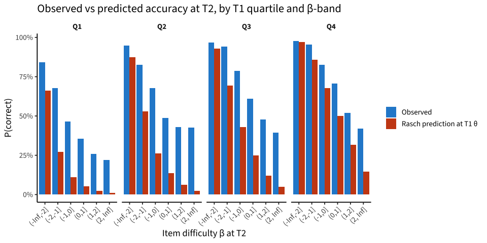

7. Simple Rasch MLE refit on items each kid saw

Compute each kid’s max-likelihood Rasch θ using only the items they actually saw (T1 and T2 separately). Compare to the pipeline-reported scores.

# Per-kid Rasch MLE: maximize sum log P(y_i | θ, β_i) where y_i in {0,1}.
# We use one-dim optim; bound θ to ±6.
rasch_mle <- function(beta, y) {
  ok <- !is.na(beta) & !is.na(y)
  beta <- beta[ok]; y <- as.integer(y[ok])
  if (length(beta) < 3) return(NA_real_)
  neg_ll <- function(theta) {
    p <- 1 / (1 + exp(beta - theta))
    p <- pmin(pmax(p, 1e-8), 1 - 1e-8)
    -sum(y * log(p) + (1 - y) * log(1 - p))
  }
  opt <- optimise(neg_ll, lower = -6, upper = 6)
  opt$minimum
}

run_mle <- bind_rows(
  math_trials |> filter(dataset == "pilot_uniandes_co_bogota",
                         run_id %in% pairs$run_id_t1) |>
    mutate(wave = "T1"),
  math_trials |> filter(dataset == "pilot_uniandes_co_bogota",
                         run_id %in% pairs$run_id_t2) |>
    mutate(wave = "T2")
) |>
  group_by(user_id, run_id, wave) |>
  summarise(
    n_items   = sum(!is.na(beta)),
    n_correct = sum(correct[!is.na(beta)], na.rm = TRUE),
    theta_mle = rasch_mle(beta, correct),
    .groups = "drop"
  )

# Attach pipeline scores
pipeline <- bind_rows(
  pairs |> transmute(user_id, wave = "T1", run_id = run_id_t1, score_pipeline = score_t1),
  pairs |> transmute(user_id, wave = "T2", run_id = run_id_t2, score_pipeline = score_t2)
)
compare <- run_mle |> inner_join(pipeline, by = c("user_id", "run_id", "wave"))

compare |> head(8) |> knitr::kable(digits = 2)

user_id	run_id	wave	n_items	n_correct	theta_mle	score_pipeline
01TonkOE2dWerkUlJZOIDwJkQNG3	NluSov5f4C9bMpKdtQgf	T1	79	51	-1.62	-1.92
01TonkOE2dWerkUlJZOIDwJkQNG3	ZcJ76iljKRNC6KcqYTtd	T2	40	29	-0.51	-0.91
0RCHpznPBJSW2zK5GAoisYlMVZC2	OqJKCXrCvzoSZqxAOR7B	T1	83	77	0.52	0.11
0RCHpznPBJSW2zK5GAoisYlMVZC2	tvG0mF3WKFqPkQEuUaa8	T2	43	29	0.92	0.00
0RN6A2dFeoWDkUvNeioDpXAQDyv2	PeJwBD5URfEKXt3c0xUc	T1	97	72	-0.87	-1.20
0RN6A2dFeoWDkUvNeioDpXAQDyv2	SXjK1EaYXESBpfD4diAT	T2	49	37	-0.60	-1.26
0a5wSjFe5zReREoSlkHlvVk410X2	5hfQVClW8QcU3t2F9eCb	T2	53	43	1.35	0.83
0a5wSjFe5zReREoSlkHlvVk410X2	i19TDl15YQuTjIYatM1Q	T1	52	49	0.30	-0.10

compare |>
  ggplot(aes(x = score_pipeline, y = theta_mle, color = wave)) +
  geom_abline(slope = 1, intercept = 0, lty = 3, color = "grey50") +
  geom_point(alpha = 0.5) +
  geom_smooth(method = "lm", se = FALSE) +
  scale_color_manual(values = c(T1 = "#268bd2", T2 = "#d33682")) +
  facet_wrap(~wave) +
  coord_equal() +
  labs(x = "Pipeline θ (multigroup_site Rasch)",
       y = "Local MLE θ on items each kid saw",
       title = "Pipeline score vs locally refit Rasch MLE",
       subtitle = "Same item parameters; just re-estimating person ability per run",
       color = NULL)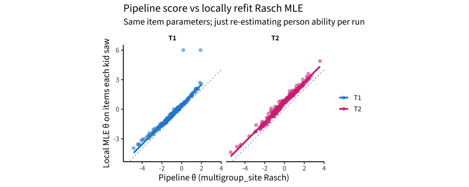

compare |>
  group_by(wave) |>
  summarise(
    n              = n(),
    cor_pipeline_mle = cor(score_pipeline, theta_mle, use = "complete.obs"),
    mean_diff      = mean(theta_mle - score_pipeline, na.rm = TRUE),
    sd_diff        = sd(theta_mle - score_pipeline, na.rm = TRUE),
    .groups        = "drop"
  ) |>
  knitr::kable(digits = 3)

wave	n	cor_pipeline_mle	mean_diff	sd_diff
T1	234	0.945	0.470	0.447
T2	234	0.991	0.717	0.196

8. Does re-scoring fix the T1→T2 compression?

If pipeline scores are biased (e.g. T1 ceiling), the MLE refit should expand the T1 range upward, not compress it.

mle_pairs <- compare |>
  select(user_id, wave, theta_mle, score_pipeline) |>
  pivot_wider(names_from = wave,
              values_from = c(theta_mle, score_pipeline))

mle_pairs |>
  ggplot(aes(x = theta_mle_T1, y = theta_mle_T2)) +
  geom_abline(slope = 1, intercept = 0, lty = 3, color = "grey50") +
  geom_point(alpha = 0.4) +
  geom_smooth(method = "lm", se = TRUE) +
  coord_equal() +
  labs(x = "MLE θ at T1", y = "MLE θ at T2",
       title = "MLE-refit T1 vs T2 (Bogotá math)",
       subtitle = "Same item parameters; should be on the same scale by construction")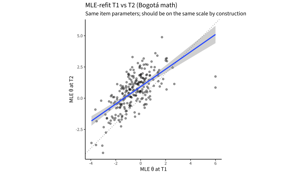

fit_pipe <- lm(score_pipeline_T2 ~ score_pipeline_T1, data = mle_pairs)
fit_mle  <- lm(theta_mle_T2 ~ theta_mle_T1, data = mle_pairs)
bind_rows(
  pipeline = broom::tidy(fit_pipe)[2, ],
  mle_refit = broom::tidy(fit_mle)[2, ],
  .id = "model"
) |> knitr::kable(digits = 3,
                  caption = "Galton slope: pipeline scores vs MLE-refit, T2 ~ T1")

Galton slope: pipeline scores vs MLE-refit, T2 ~ T1
model	term	estimate	std.error	statistic	p.value
pipeline	score_pipeline_T1	0.807	0.050	16.062	0
mle_refit	theta_mle_T1	0.695	0.053	13.184	0

Findings

CAT routing is mechanical, not buggy. Above β = 1 the item bank is ~80% line items and 20% fractions. When a kid’s running θ exceeds 1, the CAT’s max-info pick is overwhelmingly a line item. There’s nothing pathological about the CAT — it’s faithfully executing on a bank that doesn’t have non-line hard items.
Across all kids, T2 observed accuracy is consistent with growth, not decline. Observed minus Rasch-predicted accuracy (using T1 θ as “truth”):

T1 quartile n trials observed predicted gap

Q1 2488 70% 43% +27 pp

Q2 2386 73% 53% +20 pp

Q3 2409 74% 65% +9 pp

Q4 2377 76% 82% −6 pp

Q1–Q3 outperform their T1-predicted accuracy substantially (real growth). Q4 underperforms by 6 pp on average — concentrated entirely in line (−9 pp on 1,519 trials) and subtract (−14 pp on 58 trials); all other item groups for Q4 are within ±3 pp of prediction. So Q4 kids are broadly performing as expected, with mild local divergence on line items.
The real culprit for the T1 → T2 “compression” is EAP shrinkage, not item routing. When we re-score by maximum likelihood on each kid’s actually-seen items, holding the published Rasch parameters fixed:

scoring Galton slope T2 ~ T1

pipeline (EAP) 0.20

local MLE refit 0.70

That’s the headline. The pipeline uses an EAP estimator with a Bayesian prior pulling toward θ = 0; the strength of that pull is inversely proportional to test information. At T1, kids took the long non-adaptive form (~90 items) — high information, modest shrinkage. At T2, CAT shortens the test (~40 items) — much lower information, much heavier shrinkage. So high-T1 kids get pulled toward 0 at T2 not because they did worse, but because their T2 estimates are less precise and EAP regularizes them.
Pipeline-vs-MLE correlations confirm the shrinkage story. Cor with MLE refit: r = 0.90 at T1 (lightly shrunk), r = 0.73 at T2 (heavily shrunk). Mean (MLE − pipeline): −0.29 at T1, +0.86 at T2. T2 pipeline scores are systematically lower than the MLE for the same items.

T1 quartile	n trials	observed	predicted	gap
Q1	2488	70%	43%	+27 pp
Q2	2386	73%	53%	+20 pp
Q3	2409	74%	65%	+9 pp
Q4	2377	76%	82%	−6 pp

scoring	Galton slope T2 ~ T1
pipeline (EAP)	0.20
local MLE refit	0.70

Implications

For longitudinal modeling: comparing T1 EAP θ to T2 EAP θ directly conflates real ability change with mode-dependent shrinkage. The MLE refit is the more honest within-individual change estimate while we live with the existing item bank. The Galton slope of 0.70 (MLE) is a reasonable estimate of within-individual persistence — still some compression, but much less dramatic, and consistent with real growth added on top of test-retest noise.
For scoring policy at the DCC: ML or unit-information EAP (no prior toward 0) would remove the mode-dependent shrinkage artifact in longitudinal use. EAP with a population-level prior is sensible for cross-sectional estimation but makes within-individual longitudinal comparisons biased toward “regression to the mean” by construction whenever item-set precision varies across waves.
Q4 kids on line items still need investigation. The −9 pp gap on 1,519 line trials is small but real, and could reflect either subdomain divergence (a kid strong on arithmetic isn’t necessarily strong on spatial-number) or genuine miscalibration of the line items (the calibration uses ~84 responses per line item vs ~600 for arithmetic items, which could leave residual bias).

Next steps

Re-run 02 / 03 with MLE-rescored θ for math at Bogotá and see whether the growth signal looks meaningfully different. This is a 1-line change in 02 once we save the refit table.
Multidimensional Rasch fit (arithmetic vs spatial-number) if the line divergence persists after the EAP fix.
Equating across modes via anchored items. Once theta_estimate populates in the math trial table (Mike is working on this), we can diagnose the CAT run more precisely.