Corrected longitudinal trajectories — math & vocab, CO & DE

AI-generated — not for publication

The code and prose in this chapter were written by Claude Code (an AI coding agent) under human direction. They have not been line-by-line verified by a human and must not be published or cited as-is.

Preliminary & unvetted analysis

These are exploratory analyses of preliminary, in-progress LEVANTE data. Results have not been reviewed or validated and require checking by the LEVANTE Data Coordinating Center before any use.

Purpose

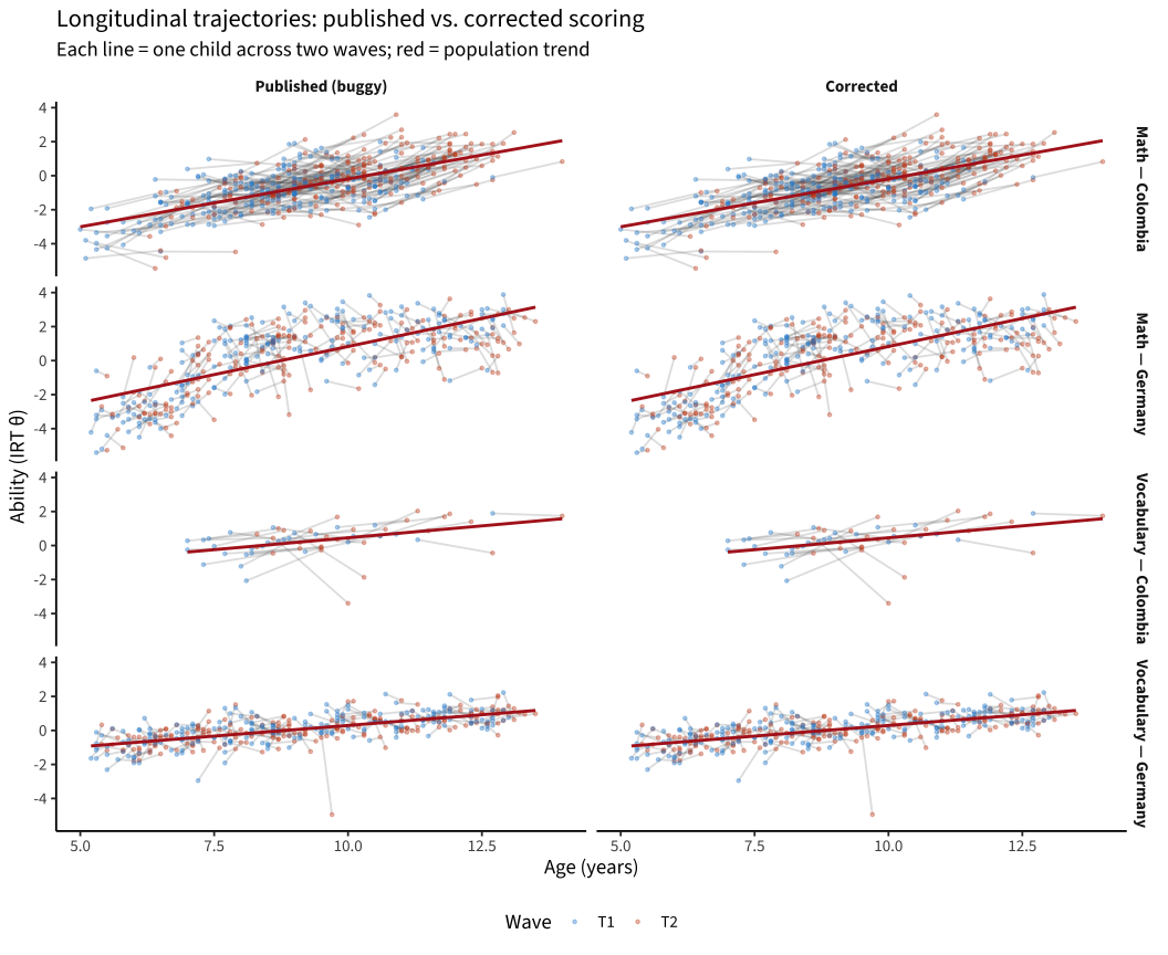
Presentation-ready before/after longitudinal trajectories for the two tasks and two sites where the column-order scoring bug mattered most. “Published” = the scores currently in levante_data_latest (buggy). “Corrected” = rescored with the column-order fix, using the same v1_14 IRT models and the same EAP estimator the pipeline uses (so this previews what the re-run pipeline will produce; WLE looks essentially identical — see tasks/math_item_calibration and the EAP/WLE checks).

High-res PNGs are written to figures/ for slides.

Code

source(here::here("common.R"))
library(rlevante)
library(mirt)
library(patchwork)

fig_dir <- here::here("figures"); fs::dir_create(fig_dir)

scores <- read_rds(here::here("data", "scores_all_sites.rds"))

cells <- tribble(
  ~task_id,    ~tk,     ~dataset,                   ~site,      ~model_file,
  "egma-math", "math",  "pilot_uniandes_co_bogota", "Colombia", "math_model_record_v1_14.rds",
  "egma-math", "math",  "pilot_mpieva_de_main",     "Germany",  "math_model_record_v1_14.rds",
  "vocab",     "vocab", "pilot_uniandes_co_bogota", "Colombia", "vocab_model_co_v1_14.rds",
  "vocab",     "vocab", "pilot_mpieva_de_main",     "Germany",  "vocab_model_de_v1_14.rds"
)

Code

rescore_cell <- function(task_id, tk, dataset, model_file, ...) {
  mod_rec <- read_rds(here::here("data", model_file))
  tr <- load_levante_trials(task_ids = task_id) |> filter(dataset == !!dataset)
  score_with_method(tr, tk, dataset, method = "EAP", mod_rec = mod_rec) |>
    transmute(run_id, score_corrected = score)
}

corrected <- cells |>
  mutate(scored = pmap(cells, rescore_cell)) |>
  select(task_id, dataset, scored) |>
  unnest(scored)

# Assemble: published (buggy) + corrected, with age/wave per run
traj <- scores |>
  filter(task_id %in% cells$task_id, dataset %in% cells$dataset) |>
  select(run_id, user_id, age, task_id, task_label, dataset,
         score_published = score) |>
  inner_join(cells |> distinct(task_id, dataset, site),
             by = c("task_id", "dataset")) |>
  left_join(corrected, by = c("run_id", "task_id", "dataset")) |>
  group_by(task_id, dataset, user_id) |>
  arrange(age) |> mutate(wave = row_number()) |> ungroup() |>
  filter(wave <= 2)

# keep only kids with two waves
two_wave <- traj |>
  group_by(task_id, dataset, user_id) |>
  filter(n_distinct(wave) == 2) |> ungroup() |>
  mutate(cell = paste0(task_label, " — ", site))

Before / after trajectories (age on x)

Code

plot_long <- two_wave |>
  pivot_longer(c(score_published, score_corrected),
               names_to = "scoring", values_to = "theta") |>
  mutate(scoring = recode(scoring,
                          score_published = "Published (buggy)",
                          score_corrected = "Corrected") |>
           factor(levels = c("Published (buggy)", "Corrected")),
         theta = pmin(pmax(theta, -6), 6))

p_traj <- ggplot(plot_long, aes(x = age, y = theta)) +
  geom_line(aes(group = user_id), alpha = 0.18, color = "grey30") +
  geom_point(aes(color = factor(wave)), alpha = 0.35, size = 0.8) +
  geom_smooth(method = "lm", se = FALSE, color = "firebrick", linewidth = 1) +
  facet_grid(cell ~ scoring) +
  scale_color_manual(values = c(`1` = "#268bd2", `2` = "#cb4b16"),
                     name = "Wave", labels = c("T1", "T2")) +
  labs(x = "Age (years)", y = "Ability (IRT θ)",
       title = "Longitudinal trajectories: published vs. corrected scoring",
       subtitle = "Each line = one child across two waves; red = population trend") +
  theme(legend.position = "bottom")
p_traj

Code

ggsave(file.path(fig_dir, "trajectories_before_after.png"), p_traj,
       width = 11, height = 9, dpi = 300, bg = "white")

T1 vs T2 scatter (the compression, before/after)

Code

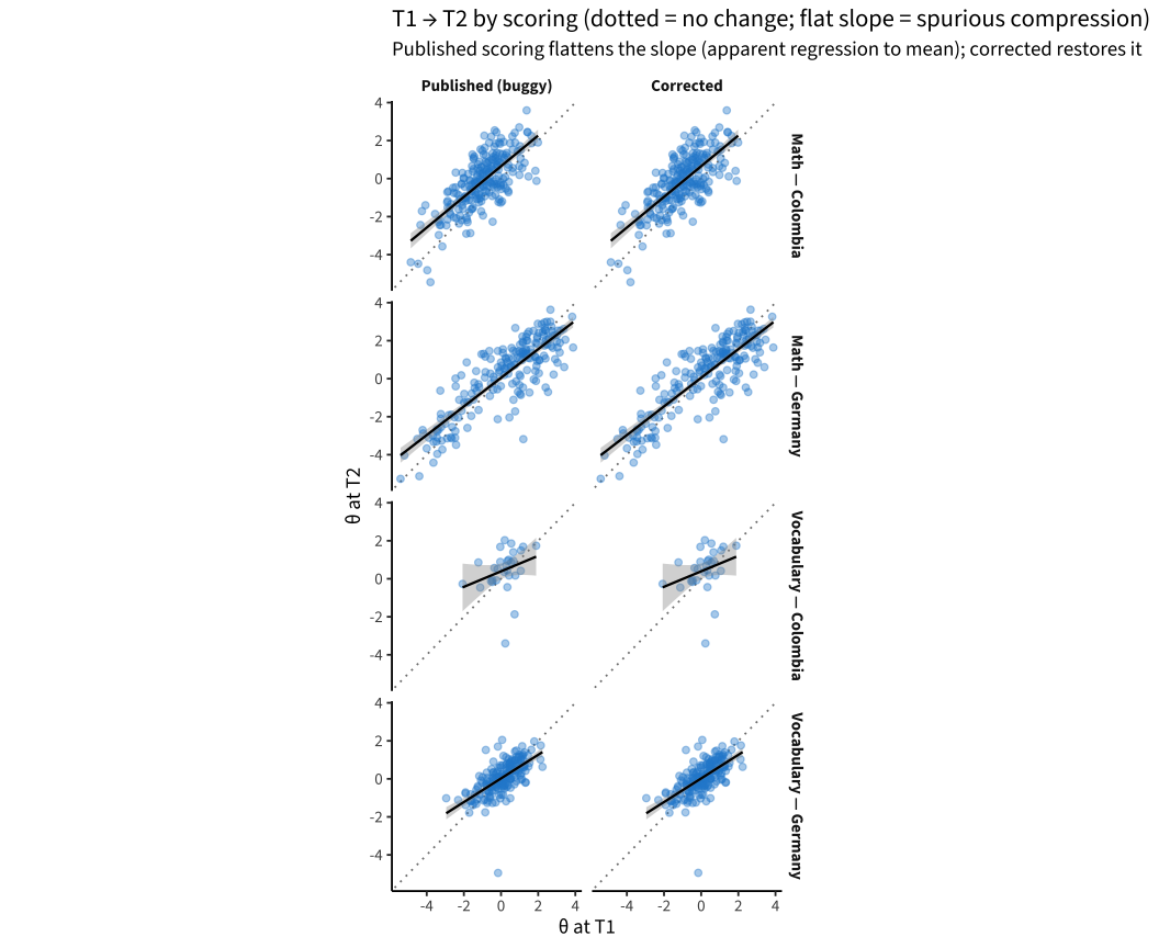
pairs <- two_wave |>
  select(cell, user_id, wave, score_published, score_corrected) |>
  pivot_longer(c(score_published, score_corrected),
               names_to = "scoring", values_to = "theta") |>
  mutate(scoring = recode(scoring, score_published = "Published (buggy)",
                          score_corrected = "Corrected")) |>
  pivot_wider(names_from = wave, values_from = theta, names_prefix = "t") |>
  mutate(scoring = factor(scoring, levels = c("Published (buggy)", "Corrected")),
         t1 = pmin(pmax(t1, -6), 6), t2 = pmin(pmax(t2, -6), 6))

p_scatter <- ggplot(pairs, aes(x = t1, y = t2)) +
  geom_abline(slope = 1, intercept = 0, lty = 3, color = "grey50") +
  geom_point(alpha = 0.4, color = "#268bd2") +
  geom_smooth(method = "lm", se = TRUE, color = "black", linewidth = 0.8) +
  facet_grid(cell ~ scoring) +
  coord_equal() +
  labs(x = "θ at T1", y = "θ at T2",
       title = "T1 → T2 by scoring (dotted = no change; flat slope = spurious compression)",
       subtitle = "Published scoring flattens the slope (apparent regression to mean); corrected restores it") +
  theme(aspect.ratio = 1)
p_scatter

Code

ggsave(file.path(fig_dir, "t1_t2_scatter_before_after.png"), p_scatter,
       width = 11, height = 9, dpi = 300, bg = "white")

Summary table

Code

pairs |>
  group_by(cell, scoring) |>
  summarise(n = n(),
            mean_change = mean(t2 - t1, na.rm = TRUE),
            galton_slope = coef(lm(t2 ~ t1))[2],
            .groups = "drop") |>
  pivot_wider(names_from = scoring,
              values_from = c(n, mean_change, galton_slope)) |>
  knitr::kable(digits = 2)

cell	n_Published (buggy)	n_Corrected	mean_change_Published (buggy)	mean_change_Corrected	galton_slope_Published (buggy)	galton_slope_Corrected
Math — Colombia	234	234	0.85	0.85	0.81	0.81
Math — Germany	200	200	-0.01	-0.01	0.75	0.75
Vocabulary — Colombia	30	30	0.29	0.29	0.41	0.41
Vocabulary — Germany	202	202	0.00	0.00	0.62	0.62

Code

write_rds(two_wave, here::here("data", "corrected_trajectories_long.rds"))

Figures saved to figures/trajectories_before_after.png and figures/t1_t2_scatter_before_after.png.