Shape Rotation (Mental Rotation) — the angle effect and item validity
ImportantAI-generated — not for publication
The code and prose in this chapter were written by Claude Code (an AI coding agent) under human direction. They have not been line-by-line verified by a human and must not be published or cited as-is.
WarningPreliminary & unvetted analysis
These are exploratory analyses of preliminary, in-progress LEVANTE data. Results have not been reviewed or validated and require checking by the LEVANTE Data Coordinating Center before any use.
Question
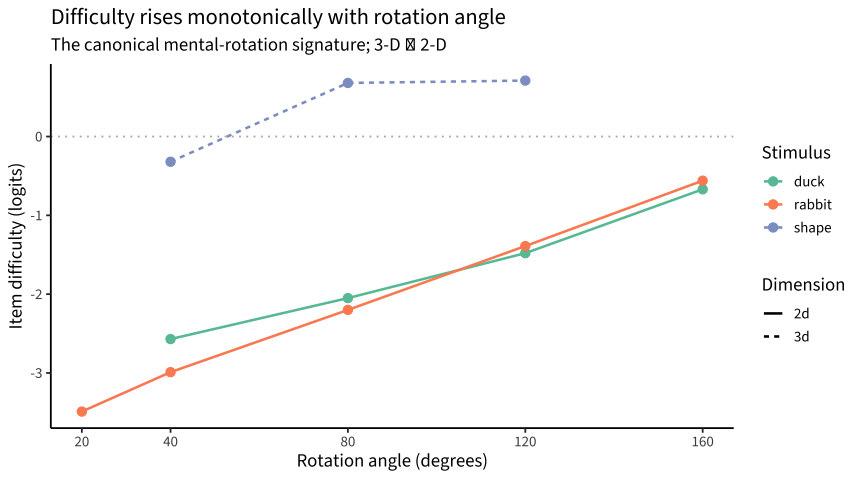
Shape Rotation (mental rotation) asks the child to pick which of two silhouettes matches a target when rotated. The canonical mental-rotation signature is that difficulty (and RT) increases monotonically with the rotation angle, and that 3-D figures are harder than 2-D. If the LEVANTE item difficulties show this, it’s strong evidence the task measures what it should. Item structure: mrot_{2d|3d}_{stimulus}_{angle}.
ip |>ggplot(aes(x = angle, y = difficulty, color = stim, group = stim)) +geom_hline(yintercept =0, lty =3, color ="grey70") +geom_line(aes(linetype = dim), linewidth =0.9) +geom_point(size =2.8) +scale_color_brewer(palette ="Set2") +scale_x_continuous(breaks =c(20,40,80,120,160)) +labs(x ="Rotation angle (degrees)", y ="Item difficulty (logits)",title ="Difficulty rises monotonically with rotation angle",subtitle ="The canonical mental-rotation signature; 3-D ≫ 2-D",color ="Stimulus", linetype ="Dimension")
Code
ip |>group_by(dim) |>summarise(n_items =n(),cor_angle_difficulty =cor(angle, difficulty),logits_per_45deg =coef(lm(difficulty ~ angle))[2] *45,mean_discrimination =mean(discrimination),.groups ="drop") |> knitr::kable(digits =3,caption ="Angle effect by dimension (difficulty near-linear in angle)")
Angle effect by dimension (difficulty near-linear in angle)
dim
n_items
cor_angle_difficulty
logits_per_45deg
mean_discrimination
2d
9
0.988
0.855
1.753
3d
3
0.879
0.579
1.017
The difficulty ordering is almost perfectly determined by rotation angle (2-D r ≈ 0.99, 3-D r ≈ 0.88), increasing ~0.85 logits per 45° for 2-D figures. 3-D figures are much harder and shifted up. This is exactly the mental-rotation effect — a clean validity result.
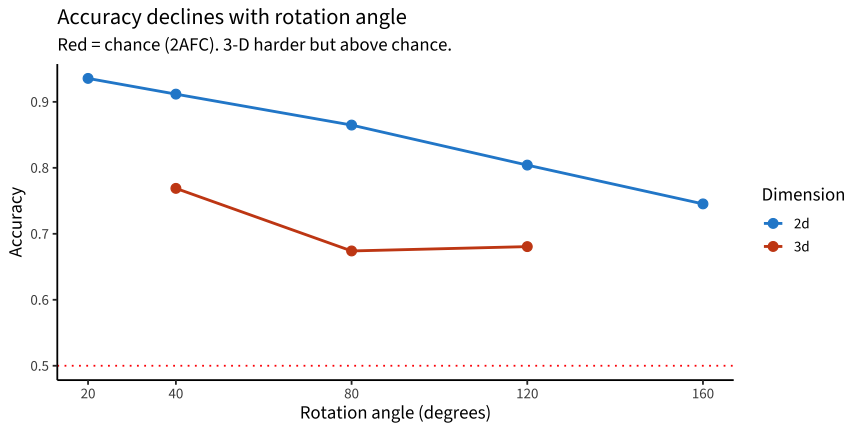
2. Accuracy by angle (the classic curve)
Code
tr <-load_levante_trials(task_ids ="mental-rotation") |>mutate(correct =as.numeric(correct),dim =str_extract(item_uid, "2d|3d"),angle =as.integer(str_extract(item_uid, "[0-9]+$")))tr |>filter(!is.na(dim), !is.na(angle), item_uid %in% ip$item_uid) |>group_by(dim, angle) |>summarise(acc =mean(correct, na.rm =TRUE), n =n(), .groups ="drop") |>ggplot(aes(x = angle, y = acc, color = dim)) +geom_hline(yintercept =0.5, lty =3, color ="red") +geom_line(linewidth =1) +geom_point(size =3) +scale_color_manual(values =c(`2d`="#268bd2", `3d`="#cb4b16")) +scale_x_continuous(breaks =c(20,40,80,120,160)) +labs(x ="Rotation angle (degrees)", y ="Accuracy",title ="Accuracy declines with rotation angle",subtitle ="Red = chance (2AFC). 3-D harder but above chance.",color ="Dimension")
tr |>filter(!item_uid %in% ip$item_uid) |>count(item_uid, name ="n_trials") |>arrange(desc(n_trials)) |> knitr::kable(caption ="Items present in data but not calibrated (low-n polygon stimuli)")
Items present in data but not calibrated (low-n polygon stimuli)
item_uid
n_trials
mrot_2d_polygon1_160
66
mrot_2d_polygon1_120
59
mrot_2d_polygon2_160
42
mrot_2d_polygon1_080
29
mrot_2d_polygon2_120
15
mrot_2d_polygon2_080
14
mrot_2d_polygon1_040
6
mrot_2d_polygon2_040
4
Eight extra 2-D polygon stimuli appear in the data but weren’t calibrated — all very low-n (≤ 66 trials). Discrimination is healthy for 2-D (≈ 1.5–2.6, higher at larger angles) and lower for 3-D (≈ 0.9–1.2), consistent with 3-D being harder and noisier.
Preliminary: are the new polygons “intermediate”?
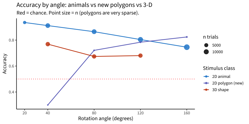
The polygons are new stimuli intended to sit between the 2-D animals (easy) and the 3-D shapes (hard). A quick accuracy-by-angle look across the three stimulus classes:
Code
cls <- tr |>mutate(angle =as.integer(str_extract(item_uid, "[0-9]+$")),klass =case_when(str_detect(item_uid, "polygon") ~"2D polygon (new)",str_detect(item_uid, "_2d_") ~"2D animal",str_detect(item_uid, "_3d_") ~"3D shape")) |>filter(!is.na(angle), !is.na(klass)) |>group_by(klass, angle) |>summarise(acc =mean(correct, na.rm =TRUE), n =n(), .groups ="drop")cls |>ggplot(aes(x = angle, y = acc, color = klass, group = klass)) +geom_hline(yintercept =0.5, lty =3, color ="red") +geom_line(linewidth =0.9) +geom_point(aes(size = n), alpha =0.85) +scale_color_manual(values =c("2D animal"="#268bd2","2D polygon (new)"="#6c71c4","3D shape"="#cb4b16")) +scale_x_continuous(breaks =c(20,40,80,120,160)) +labs(x ="Rotation angle (degrees)", y ="Accuracy",title ="Accuracy by angle: animals vs new polygons vs 3-D",subtitle ="Red = chance. Point size = n (polygons are very sparse).",color ="Stimulus class", size ="n trials")
Caveat — and a flag. With only 10–108 trials per polygon cell this is preliminary, but two things stand out: (1) the polygons do not sit cleanly between animals and 3-D — at large angles their accuracy (≈ 0.78–0.82) is near the animals and above the 3-D shapes; and (2) polygon accuracy rises with angle (0.30 at 40° → 0.82 at 160°), the reverse of the normal mental-rotation effect seen for animals and 3-D. The 40° point is just 10 trials, so this could be noise — but a reversed angle gradient on a new stimulus warrants checking the polygon items (answer keys / rotation rendering) and gathering more data before calibrating them in.
Shape Rotation is a clean, valid measure. Item difficulty shows the canonical mental-rotation angle effect (near-linear, r ≈ 0.99 for 2-D), with 3-D figures appropriately harder.
2PL discriminations are healthy; the model fits the design.
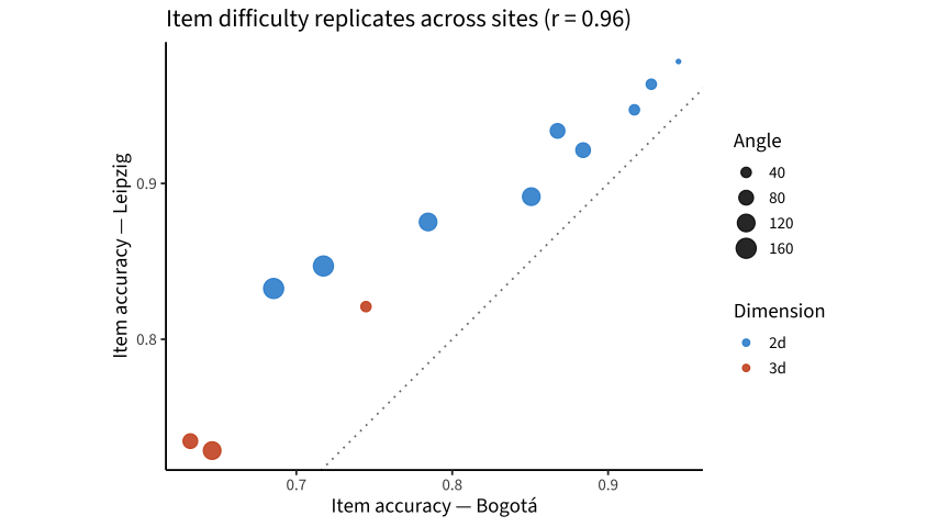
Difficulty replicates across sites (r ≈ 0.96).
Only housekeeping issue: a few low-n polygon stimuli are uncalibrated and should be excluded from scoring.
No scoring concerns — usable as-is for growth/SEM.