The code and prose in this chapter were written by Claude Code (an AI coding agent) under human direction. They have not been line-by-line verified by a human and must not be published or cited as-is.
WarningPreliminary & unvetted analysis
These are exploratory analyses of preliminary, in-progress LEVANTE data. Results have not been reviewed or validated and require checking by the LEVANTE Data Coordinating Center before any use.
The question
What latent structure organizes the nine core tasks — and can we trust that structure across age and site? Picking a factor model from the data is deceptively hard here because three things are entangled:
The structure changes developmentally (factors differentiate with age).
Sites may not share the structure (different languages, populations, administration), and Bogotá’s partial battery leaves some task pairs with no joint coverage.
Single indicators — most LEVANTE constructs are one task, so a task’s reliable specific variance is confounded with error; we cannot even ask “is ToM separable?” without separating the two.
The discipline that organizes this: measurement before structure. “3 factors vs 2,” “factors differentiate with age,” “Bogotá differs” can all be measurement non-invariance masquerading as structure. So we (a) disattenuate to handle the single-indicator problem, (b) select a structure, then (c) test whether its measurement model is invariant across site and age before trusting any structural claim. (Notebook 04 complements this with the exploratory ESEM and the smooth age-differentiation curves; here we are confirmatory.)
(The previous version of this notebook — construct-level latent growth curves — is preserved at old/03_sem_growth_lgc.qmd.)
Code
source(here::here("common.R"))library(lavaan)library(tidySEM)sc <-read_rds(here("data/scores_all_sites.rds"))sites4 <-c("pilot_mpieva_de_main","pilot_uniandes_co_bogota","pilot_uniandes_co_rural","pilot_western_ca_main")core <-c("matrix","mrot","math","hf","mg","sds","trog","vocab","tom")fitm <-function(f, m) as.numeric(fitMeasures(f, m))heywood <-function(f){ pe <-parameterEstimates(f)any(pe$est[pe$op=="~~"& pe$lhs==pe$rhs] <-1e-4) ||any(abs(subset(standardizedSolution(f), op=="=~")$est.std) >1.001) }
Pooled cross-sectional sample (first observation per child, four data-rich sites): N = 2151. Per-task marginal reliabilities (from the EAP SEs) range 0.79–0.93.
1. The single-indicator problem: disattenuated task correlations
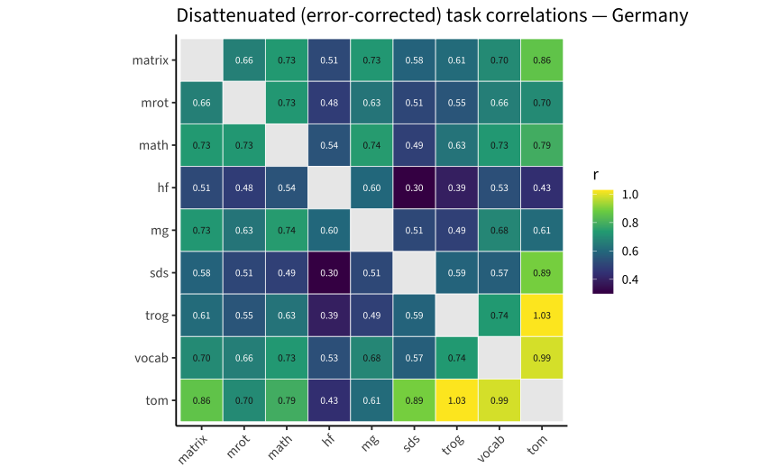
To ask whether any task carries reliable variance distinct from the others, we first strip measurement error. Each task becomes a single-indicator latent with its error variance fixed from its reliability (eta_t =~ 1*t; t ~~ (1−ρ_t)·t, scores standardized), and we read off the error-corrected correlations. We use Germany (the complete-battery site) to avoid coverage gaps.
ToM is not separable. Error-corrected, it correlates ≈ 0.90 with TROG and ≈ 0.86 with vocab — its reliable variance is essentially the verbal/language cluster, leaving little room for an independent “social cognition” construct at the task level.
The most distinct task is Hearts & Flowers (lowest correlations, ≈ 0.3–0.6) — the inhibition/EF task carries the most reliable variance not shared with the rest. Even so, every off-diagonal is positive and large: a strong positive manifold.
2. Which structure? (confirmatory comparison)
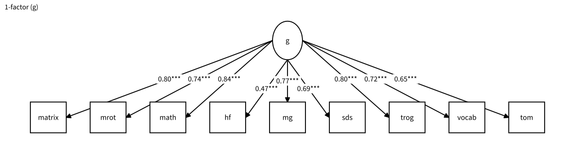
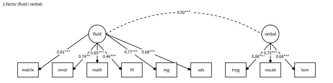
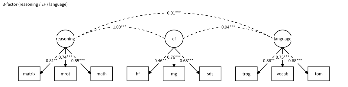
We compare a single general factor (g), the emergent 2-factor (fluid / verbal), the theory 3-factor (reasoning / EF / language), and a bifactor (g + orthogonal domain specifics) — standard CFA, pooled (FIML), age partialled. Because a strong positive manifold makes fit indices keep nudging toward more (near-collinear, often improper) factors, we read the table by propriety first, then parsimony (BIC), then fit.
The bifactor is improper (a Heywood case — its specific factors collapse/explode), itself a finding: beyond g, domain-specific variance is negligible. Among the proper models the 2-factor (fluid/verbal) is BIC-preferred (BIC 27947 vs 3-factor 27968 vs g 28023, on the 2026-08 N = 2,151 sample) and ties the 3-factor on fit (CFI ≈ 0.91) — the third factor does not earn its parsimony cost. And the 3-factor’s factors are near-collinear (reasoning–EF ≈ 0.99). So the honest read is a dominant general factor with ~two weakly-separable domains (“g plus modest domains”), consistent with 04’s ESEM. (Relative to the June render — N = 2,063, BIC 25638/25657/25708, reasoning–EF 0.96 — the added rural children left the model ordering intact and made the fluid factors more collinear.) We carry the proper candidates (g / 2-factor / 3-factor) into the invariance tests.
The three proper candidates as path diagrams (standardized loadings, pooled cross-sectional). The curved arrows between latent factors show how strongly the domains correlate — visibly near-collinear in the 2- and 3-factor models.
Code
obs <-c("matrix","mrot","math","hf","mg","sds","trog","vocab","tom")diag_specs <-list(list(nm ="1-factor (g)", mod ="g =~ matrix+mrot+math+hf+mg+sds+trog+vocab+tom",top =c("","","","","g","","","","")),list(nm ="2-factor (fluid / verbal)", mod ="fluid =~ matrix+mrot+math+hf+mg+sds\n verbal =~ trog+vocab+tom",top =c("","","fluid","","","","","verbal","")),list(nm ="3-factor (reasoning / EF / language)",mod ="reasoning =~ matrix+mrot+math\n ef =~ hf+mg+sds\n language =~ trog+vocab+tom",top =c("","reasoning","","","ef","","","language","")))for (s in diag_specs) { f <-cfa(s$mod, xw, std.lv =TRUE, missing ="fiml") lay <-do.call(get_layout, c(as.list(c(s$top, obs)), rows =2)) gg <-prepare_graph(f, layout = lay)edges(gg) <-edges(gg) |>filter(from != to) # loadings + factor correlations only (drop variances)nodes(gg) <-nodes(gg) |>mutate(label = name) # node names onlyprint(plot(gg) +labs(title = s$nm) +theme(plot.title =element_text(size =11)))}
Robustness: adding the ROAR reading tasks
ROAR (word / sentence / phoneme) reading isn’t a LEVANTE core task and its site coverage is uneven, so it stays out of the invariance ladders below (and out of the disattenuated matrix — Germany has no ROAR-phoneme data, and ROAR-Sentence carries no model-based SE). But we can add it to the pooled structure comparison to ask: does the 2-factor hold with reading, and is reading separable?
With reading added, a separate reading factor is BIC-justified (3-factor BIC 36297 < 2-factor 36358 < g 36465) — three reading indicators carry enough distinct variance to cohere. But it sits squarely in the positive manifold: reading correlates ≈ 0.85 with verbal and ≈ 0.87 with fluid — about equally with both, i.e. it relates to the general factor rather than specifically to language (echoing 04, where reading relates to g about as much as to language). So reading is a weakly-separable sub-domain — BIC-justified once it has three indicators, but near-collinear with everything; the “g + a couple of modest domains” reading is unchanged.
Age effects on the abilities
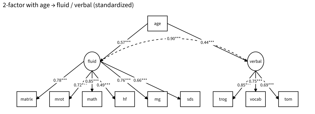
Regressing standardized age onto each latent shows how strongly — and how differently — the abilities grow (measurement model + age regressions).
Code
age_mods <-list(`g`="g =~ matrix+mrot+math+hf+mg+sds+trog+vocab+tom\n g ~ age_c",`2-factor`="fluid =~ matrix+mrot+math+hf+mg+sds\n verbal =~ trog+vocab+tom\n fluid ~ age_c\n verbal ~ age_c",`3-factor`="reasoning =~ matrix+mrot+math\n ef =~ hf+mg+sds\n language =~ trog+vocab+tom\n reasoning ~ age_c\n ef ~ age_c\n language ~ age_c")afits <-map(age_mods, ~cfa(.x, xw, std.lv =TRUE, missing ="fiml"))imap_dfr(afits, ~standardizedSolution(.x) |>filter(op =="~") |>transmute(model = .y, latent = lhs, `age effect (std)`=round(est.std, 3), p =round(pvalue, 3))) |> knitr::kable(caption ="Standardized age → latent effects (cross-sectional)")
Standardized age → latent effects (cross-sectional)
model
latent
age effect (std)
p
g
g
0.544
0
2-factor
fluid
0.571
0
2-factor
verbal
0.442
0
3-factor
reasoning
0.574
0
3-factor
ef
0.554
0
3-factor
language
0.442
0
Code
obs <-c("matrix","mrot","math","hf","mg","sds","trog","vocab","tom")lay <-do.call(get_layout, c(as.list(c(c("","","","","age_c","","","",""),c("","","fluid","","","","","verbal",""), obs)), rows =3))ssol <-standardizedSolution(afits[["2-factor"]]) # show standardized estimatesgg <-prepare_graph(afits[["2-factor"]], layout = lay)e <-edges(gg) |>filter(from != to)e$label <-map2_chr(e$from, e$to, function(a, b){ r <- ssol |>filter((lhs == a & rhs == b) | (lhs == b & rhs == a))if (nrow(r) ==0) return(NA_character_) sig <-ifelse(r$pvalue[1] < .001, "***", ifelse(r$pvalue[1] < .01, "**", ifelse(r$pvalue[1] < .05, "*", "")))sprintf("%.2f%s", r$est.std[1], sig) })edges(gg) <- enodes(gg) <-nodes(gg) |>mutate(label =ifelse(name =="age_c", "age", name))print(plot(gg) +labs(title ="2-factor with age → fluid / verbal (standardized)"))
Both abilities rise steeply with age, but fluid grows faster than verbal (standardized age effects ≈ 0.57 vs 0.47). That differential growth is part of why they de-correlate: if the fluid core accelerates relative to verbal across childhood, the two pull apart — the structural side of the same coin as 04’s falling fluid–verbal correlation. (The reasoning/EF/language 3-factor shows the same: the fluid-side factors carry the steeper age effects.)
3. Does the structure replicate across sites?
A full all-site multigroup is blocked by Bogotá’s partial battery (zero joint coverage of some task pairs → FIML breaks). So we (a) fit each model separately per site (descriptive replication, incl. Canada), and (b) run a formal 2-group multigroup for the two sites with full mutual coverage (Germany + Canada).
Code
meas <-list(g ="g =~ matrix+mrot+math+hf+mg+sds+trog+vocab+tom",`2-factor`="fluid =~ matrix+mrot+math+hf+mg+sds\n verbal =~ trog+vocab+tom",`3-factor`="reasoning =~ matrix+mrot+math\n ef =~ hf+mg+sds\n language =~ trog+vocab+tom")grp <- xw |>mutate(site =recode(dataset, pilot_mpieva_de_main="Germany",pilot_uniandes_co_bogota="Bogotá-urban", pilot_uniandes_co_rural="Bogotá-rural", pilot_western_ca_main="Canada"))per_site <-map_dfr(unique(grp$site), function(s){ d <-filter(grp, site == s)map_dfr(meas, function(m){ f <-tryCatch(cfa(m, d, std.lv=TRUE, missing="fiml"), error=function(e) NULL)if(is.null(f)||!lavInspect(f,"converged")) return(tibble(CFI=NA, BIC=NA, max_factor_r=NA)) cr <-tryCatch(lavInspect(f,"cor.lv"), error=function(e) NULL)tibble(CFI=fitm(f,"cfi"), BIC=fitm(f,"bic"),max_factor_r =if(!is.null(cr) &&is.matrix(cr) &&ncol(cr)>1) max(cr[upper.tri(cr)]) elseNA_real_) }, .id="model") |>mutate(site = s, n =nrow(d)) })per_site |>mutate(model =factor(model, names(meas))) |>arrange(site, model) |>select(site, n, model, CFI, BIC, max_factor_r) |>mutate(across(c(CFI,max_factor_r), \(x) round(x,3)), BIC =round(BIC)) |> knitr::kable(caption ="Per-site CFA (max_factor_r = strongest inter-factor correlation): both 2- and 3-factor beat g; factors near-collinear")
Per-site CFA (max_factor_r = strongest inter-factor correlation): both 2- and 3-factor beat g; factors near-collinear
Site invariance ladders (Germany + Canada), 2- and 3-factor
model
invariance
CFI
RMSEA
dCFI
2-factor
configural
0.989
0.037
NA
2-factor
metric
0.961
0.066
-0.029
2-factor
scalar
0.828
0.131
-0.132
3-factor
configural
0.990
0.038
NA
3-factor
metric
0.973
0.057
-0.017
3-factor
scalar
0.843
0.131
-0.129
A multi-factor structure replicates in every site — both the 2- and 3-factor beat g on BIC (CFI ≈ 0.97–0.99). Notably the 2-factor stays proper everywhere (strongest factor r ≈ 0.83–0.85), whereas the 3-factor goes improper in Bogotá-rural (reasoning–EF = 1.10 > 1 — the two fluid factors are empirically indistinguishable there): another mark in the 2-factor’s favour. The Germany + Canada multigroup supports configural invariance for both (CFI ≈ 0.99), only approximate metric invariance (ΔCFI ≈ −0.029 for the 2-factor, −0.017 for the 3-factor — loadings roughly, not strictly, shared, and a touch less so for the broader 2-factor), and scalar fails decisively (ΔCFI ≈ −0.13). So across two very different sites the form is shared and loadings approximately so, but absolute score levels are not comparable (and we don’t interpret them).
4. Does the structure hold across age?
This is the crucial test for the 04 differentiation finding. If factor correlations change with age (differentiation) but loadings stay invariant, the differentiation is structural. If loadings themselves drift with age, the “differentiation” could be a measurement artifact. We test metric/scalar invariance across age bins (pooled).
Metric (loading) invariance approximately holds across age (ΔCFI ≈ −0.01 configural→metric) — the loadings barely move. Scalar fails (ΔCFI ≈ −0.03): intercepts rise with age, exactly as expected when children improve. The takeaway: the age-differentiation in 04 (factor correlations falling with age) is structural change, not loading drift — the measurement model is stable enough across age for that interpretation to stand. (See 04 for the smooth local-SEM correlation curves under 2/3/4-factor structures.)
Single indicators: disattenuating (fixed-error latents) shows the core tasks form a strong positive manifold; ToM is not separable from the verbal cluster (error-corrected r ≈ 0.9), while H&F carries the most distinct reliable variance.
Structure: a dominant general factor with ~two weakly-separable domains. Among proper models the 2-factor (fluid/verbal) is BIC-preferred, tying the 3-factor on fit and staying proper in every site (the 3-factor goes improper in Bogotá-rural, reasoning–EF > 1); the bifactor’s specifics degenerate. Consistent with 04’s ESEM.
Site: the multi-factor structure replicates across Germany, Bogotá, and Canada; the Germany + Canada multigroup supports configural and approximate metric invariance (ΔCFI ≈ −0.02 to −0.03 — form and roughly loadings shared) — but not scalar (levels not comparable).
Age: loadings are ~invariant across age (metric ΔCFI ≈ −0.01) while intercepts shift — so 04’s age-differentiation is a genuine structural change, not a measurement artifact.
Net: the appropriate model is g-with-~two-modest-domains, invariant in form and approximately in loadings across site and age, with comparability limited at the level of absolute means (scalar invariance fails for both site and age). Single-task constructs like ToM cannot be separated at the task level — testing their specific variance would need the item-level upgrade flagged in the plan.