Code
source(here::here("common.R"))
library(tidyverse)
The code and prose in this chapter were written by Claude Code (an AI coding agent) under human direction. They have not been line-by-line verified by a human and must not be published or cited as-is.
These are exploratory analyses of preliminary, in-progress LEVANTE data. Results have not been reviewed or validated and require checking by the LEVANTE Data Coordinating Center before any use.
A planning view of the whole LEVANTE network — pilots, RfP1, and RfP2 — not the analyzed data. We transcribe each funded site’s main PI, data-collection country, recruitment setting, target age range, and planned wave schedule from the Q1 2026 Advisory Committee deck (papers/Q1 LEVANTE Advisory committee meeting.pdf), write it to a CSV, and then visualize (1) the enrollment ages each study recruits and (2) the eventual age coverage the accumulated waves will produce.
source(here::here("common.R"))
library(tidyverse)Transcribed from the deck’s per-cohort tables and per-site annex cards. age_min/age_max are the recruitment age band; n_waves/cadence are the planned wave schedule; school_based marks school/classroom/daycare recruitment (vs. home, lab, online, or community-cohort). See notes for deck inconsistencies and the few cases where the cohort table and annex card disagree.
sites <- tribble(
  ~cohort,       ~pi,                ~institution,                          ~country,                       ~age_min, ~age_max, ~school_based, ~longitudinal, ~n_waves, ~cadence,    ~setting,            ~notes,
  "Pilots '23",  "Manuel Bohn",      "Leuphana University Lüneburg",        "Germany",                      5, 12, FALSE, TRUE,  3,  "annual",    "online / family",   "Psychometric pilot; >=3 testing sessions.",
  "Pilots '23",  "Julián Mariño",    "Universidad de los Andes",            "Colombia",                     5, 12, TRUE,  TRUE,  3,  "annual",    "school",            "Psychometric pilot; >=3 testing sessions.",
  "Pilots '23",  "Daniel Ansari",    "Western University",                  "Canada",                       5, 12, TRUE,  TRUE,  3,  "annual",    "school",            "Psychometric pilot; >=3 testing sessions.",
  "Pilots '23",  "Ben Domingue",     "Stanford University",                 "(secondary analysis)",         NA, NA, NA,    NA,    NA, "none",      "secondary analysis","Analyzes other sites' pilot data; no recruitment.",
  "Pilots '25",  "Manuel Bohn",      "Leuphana University Lüneburg",        "Germany",                      2, 5,  FALSE, FALSE, 1,  "none",      "home / everyday",   "Vest-camera recordings; per MZF not longitudinal (deck cited 2 waves).",
  "Pilots '25",  "Charles Nelson",   "Boston Children's Hospital",          "United States",                2, 5,  FALSE, FALSE, 1,  "none",      "lab",               "Per MZF not longitudinal (deck cited lab visits + 1-yr follow-up).",
  "Pilots '25",  "Tami Katzir",      "University of Haifa",                 "Israel",                       5, 10, TRUE,  TRUE,  3,  "annual",    "school",            "K/G1/G2 cohorts; three annual waves.",
  "Pilots '25",  "Julián Mariño",    "Universidad de los Andes",            "Colombia",                     2, 5,  TRUE,  FALSE, 1,  "none",      "daycare",           "Per MZF not longitudinal (deck cited 3 annual waves 2026-28).",
  "Pilots '25",  "Ivy Nkrumah",      "University of Cape Coast",            "Ghana",                        5, 12, TRUE,  TRUE,  3,  "annual",    "school",            "With C. Y. Kwaah; three grade-cohorts, annual.",
  "RfP1",        "Alicia Forsberg",  "University of Sheffield",             "UK",                           6, 9,  TRUE,  TRUE,  3,  "annual",    "school / online",   "Annex card lists 5-13; LEVANTE study 6-9 (used). Three annual waves.",
  "RfP1",        "Catherine Lebel",  "University of Calgary",               "Canada",                       5, 6,  FALSE, TRUE,  4,  "annual",    "home",              "PdP cohort; added at 5-6, annual to age 9. Annex lists U Alberta.",
  "RfP1",        "Rogier Kievit",    "Donders Institute (Radboud)",         "Netherlands",                  5, 9,  FALSE, TRUE,  3,  "annual",    "lab / center",      "Two discrete cohorts (SMILEY ~5, Skippy ~9); 3 annual occasions.",
  "RfP1",        "Zoe Ngo",          "Max Planck Inst. Human Development",  "Germany",                      4, 10, FALSE, TRUE,  4,  "15-month",  "lab",               "Two discrete cohorts (4 & 6); 4 time points 15 months apart.",
  "RfP1",        "Iliana Karipidis", "University of Zurich",                "Switzerland",                  5, 12, TRUE,  TRUE,  3,  "annual",    "school",            "Mono/multilingual; annual over ~3 years.",
  "RfP1",        "Cecilia Calero",   "Universidad Torcuato Di Tella",       "Argentina",                    6, 9,  TRUE,  TRUE,  3,  "annual",    "school",            "Cohorts 6-7 & 8-9, three waves each.",
  "RfP2",        "Diego Lucumí",     "Universidad de los Andes",            "Colombia",                     6, 11, TRUE,  TRUE,  3,  "annual",    "school / community","Pacific-coast / PDET municipalities; three waves.",
  "RfP2",        "Dragan Gasevic",   "Monash University",                   "Colombia",                     9, 12, TRUE,  TRUE,  5,  "biannual",  "school",            "Start age 9-10; data every 6 months (deck cites up to 4 yrs).",
  "RfP2",        "Santiago Cueto",   "GRADE",                              "Peru",                         8, 11, TRUE,  TRUE,  4,  "annual",    "school",            "1500 students / 50 schools; 4 measurement points 2026-2029.",
  "RfP2",        "Kwaku Poku Asante","Kintampo Health Research Center",     "Ghana",                        10, 12, FALSE, TRUE,  3,  "annual",    "community cohort",  "GRAPHS rural cohort; annual yrs 1-3.",
  "RfP2",        "Luciano Gasser",   "University of Teacher Education Bern", "Switzerland",                  9, 12, TRUE,  TRUE,  4,  "annual",    "school",            "BELIMA/SWING; four annual waves (T1-T4). Table says 'first graders'; card age 9-12 used.",
  "RfP2",        "Dana McCoy",       "Harvard University",                  "Peru",                         6, 8,  TRUE,  TRUE,  3,  "annual",    "school / home",     "Rural Andean RCT follow-up; LEVANTE waves at ages 6,7,8.",
  "RfP2",        "Debarati Mukherjee","Public Health Foundation of India",  "India",                        6, 10, TRUE,  TRUE,  3,  "annual",    "school / community","MAASTHI cohort; waves 6-10, 7-11, 8-12.",
  "RfP2",        "Laura Di Giunta",  "Sapienza University of Rome",         "Colombia/Ecuador/Mexico/CR",   6, 12, TRUE,  TRUE,  3,  "annual",    "school",            "Arukay, 4 countries; baseline + annual follow-ups. Deck inconsistent re Costa Rica vs Dominican Republic."
) |>
  mutate(cohort = factor(cohort, c("Pilots '23","Pilots '25","RfP1","RfP2")),
         label  = paste0(pi, " · ", cohort),
         step   = recode(cadence, annual = 1, biannual = 0.5, `15-month` = 1.25, none = NA_real_))

write_csv(sites |> select(-step, -label), here::here("09_site_coverage.csv"))
sites |> select(cohort, pi, institution, country, age_min, age_max, school_based, n_waves, cadence) |>
knitr::kable(caption = "LEVANTE funded sites (23 grants across pilots, RfP1, RfP2)")| cohort | pi | institution | country | age_min | age_max | school_based | n_waves | cadence |
|---|---|---|---|---|---|---|---|---|
| Pilots ’23 | Manuel Bohn | Leuphana University Lüneburg | Germany | 5 | 12 | FALSE | 3 | annual |
| Pilots ’23 | Julián Mariño | Universidad de los Andes | Colombia | 5 | 12 | TRUE | 3 | annual |
| Pilots ’23 | Daniel Ansari | Western University | Canada | 5 | 12 | TRUE | 3 | annual |
| Pilots ’23 | Ben Domingue | Stanford University | (secondary analysis) | NA | NA | NA | NA | none |
| Pilots ’25 | Manuel Bohn | Leuphana University Lüneburg | Germany | 2 | 5 | FALSE | 1 | none |
| Pilots ’25 | Charles Nelson | Boston Children’s Hospital | United States | 2 | 5 | FALSE | 1 | none |
| Pilots ’25 | Tami Katzir | University of Haifa | Israel | 5 | 10 | TRUE | 3 | annual |
| Pilots ’25 | Julián Mariño | Universidad de los Andes | Colombia | 2 | 5 | TRUE | 1 | none |
| Pilots ’25 | Ivy Nkrumah | University of Cape Coast | Ghana | 5 | 12 | TRUE | 3 | annual |
| RfP1 | Alicia Forsberg | University of Sheffield | UK | 6 | 9 | TRUE | 3 | annual |
| RfP1 | Catherine Lebel | University of Calgary | Canada | 5 | 6 | FALSE | 4 | annual |
| RfP1 | Rogier Kievit | Donders Institute (Radboud) | Netherlands | 5 | 9 | FALSE | 3 | annual |
| RfP1 | Zoe Ngo | Max Planck Inst. Human Development | Germany | 4 | 10 | FALSE | 4 | 15-month |
| RfP1 | Iliana Karipidis | University of Zurich | Switzerland | 5 | 12 | TRUE | 3 | annual |
| RfP1 | Cecilia Calero | Universidad Torcuato Di Tella | Argentina | 6 | 9 | TRUE | 3 | annual |
| RfP2 | Diego Lucumí | Universidad de los Andes | Colombia | 6 | 11 | TRUE | 3 | annual |
| RfP2 | Dragan Gasevic | Monash University | Colombia | 9 | 12 | TRUE | 5 | biannual |
| RfP2 | Santiago Cueto | GRADE | Peru | 8 | 11 | TRUE | 4 | annual |
| RfP2 | Kwaku Poku Asante | Kintampo Health Research Center | Ghana | 10 | 12 | FALSE | 3 | annual |
| RfP2 | Luciano Gasser | University of Teacher Education Bern | Switzerland | 9 | 12 | TRUE | 4 | annual |
| RfP2 | Dana McCoy | Harvard University | Peru | 6 | 8 | TRUE | 3 | annual |
| RfP2 | Debarati Mukherjee | Public Health Foundation of India | India | 6 | 10 | TRUE | 3 | annual |
| RfP2 | Laura Di Giunta | Sapienza University of Rome | Colombia/Ecuador/Mexico/CR | 6 | 12 | TRUE | 3 | annual |
sites |> summarise(grants = n(),
                   recruiting = sum(!is.na(age_min)),
                   longitudinal = sum(longitudinal, na.rm = TRUE),
                   school_based = sum(school_based, na.rm = TRUE),
                   countries = n_distinct(country[!is.na(age_min)])) |>
knitr::kable(caption = "Network at a glance")| grants | recruiting | longitudinal | school_based | countries |
|---|---|---|---|---|
| 23 | 22 | 19 | 15 | 13 |
The network spans 23 grants; 22 recruit new participants (Stanford does secondary analysis only), of which 19 are longitudinal and 15 use school / classroom / daycare recruitment. The figures below drop the secondary-analysis site.
# Enrollment ages recruited at baseline. Two sites recruit discrete (gapped)
# cohorts rather than a continuous band; everything else recruits across its band.
enroll_ages <- function(pi, a, b) {
  if (pi == "Rogier Kievit") c(5, 9)
  else if (pi == "Zoe Ngo")  c(4, 6)
  else a:b
}

coh <- sites |> filter(!is.na(age_min)) |>
  mutate(enroll = pmap(list(pi, age_min, age_max), enroll_ages)) |>
  select(cohort, pi, label, n_waves, step, enroll) |>
  unnest(enroll) |>
rename(enroll_age = enroll)A filled square means the study recruits children of that age at baseline. Studies are grouped by cohort and ordered by youngest age. (Kievit and Ngo recruit two discrete cohorts, so their intermediate ages are blank.)
cohort_pal <- c("Pilots '23"="#b58900","Pilots '25"="#cb4b16","RfP1"="#268bd2","RfP2"="#2aa198")
ord <- sites |> filter(!is.na(age_min)) |> arrange(cohort, age_min, age_max) |> pull(label)

coh |> mutate(label = factor(label, levels = rev(ord))) |>
  ggplot(aes(enroll_age, label, fill = cohort)) +
  geom_tile(color = "white", width = 0.92, height = 0.82) +
  scale_fill_manual(values = cohort_pal, name = NULL) +
  scale_x_continuous(breaks = 0:13, expand = expansion(add = 0.5)) +
  labs(x = "Age (years)", y = NULL,
       title = "Enrollment ages recruited by each LEVANTE study",
       subtitle = "Filled = age recruited at baseline; colour = cohort") +
  theme(legend.position = "top", panel.grid.major.y = element_blank(),
        axis.text.y = element_text(size = 8))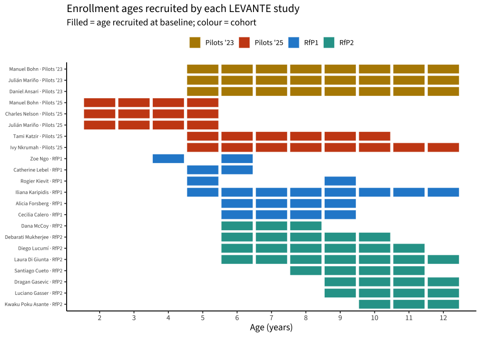
The pilots, RfP1, and RfP2 concentrate in the school-age 5–12 band, with the 2025 pilots (Bohn, Nelson, Mariño) and RfP1 Lebel anchoring early childhood (2–6) — matching the deck’s stated RfP3 priorities (transition to school; downward extension to 2–5).
Each recruited year-cohort is followed forward by its site’s planned waves (dots = waves; cadence: annual, biannual, or 15-month). Within each site the year-cohorts are stacked, so the vertical thickness shows how the overlapping waves accumulate data at each age — and the histogram below is the marginal of exactly this density.
site_order <- sites |> filter(!is.na(age_min)) |>
  arrange(cohort, age_min, age_max) |>
  mutate(base_y = n() - row_number() + 1) |>
  select(label, base_y)

coh2 <- coh |>
  arrange(label, enroll_age) |>
  group_by(label) |>
  mutate(k = n(), j = row_number(),
         offset = if_else(k == 1, 0, (j - (k + 1) / 2) / (k - 1) * 0.84)) |>
  ungroup() |>
  left_join(site_order, by = "label") |>
  mutate(y = base_y + offset,
         x_start = enroll_age,
         x_end = enroll_age + if_else(n_waves <= 1 | is.na(step), 0, (n_waves - 1) * step))

dots <- coh2 |>
  mutate(wv = map2(n_waves, step, ~ if (is.na(.x) || .x <= 1 || is.na(.y)) 0L else 0:(.x - 1))) |>
  unnest(wv) |>
  mutate(wave_age = enroll_age + if_else(is.na(step), 0, wv * step))

ggplot() +
  geom_segment(data = coh2, aes(x_start, y, xend = x_end, yend = y, color = cohort),
               linewidth = 0.5, alpha = 0.9) +
  geom_point(data = dots, aes(wave_age, y, color = cohort), size = 0.7) +
  scale_color_manual(values = cohort_pal, name = NULL) +
  scale_y_continuous(breaks = site_order$base_y, labels = site_order$label,
                     expand = expansion(add = 0.7)) +
  scale_x_continuous(breaks = 0:16, expand = expansion(add = 0.3)) +
  labs(x = "Age (years)", y = NULL,
       title = "Longitudinal coverage: each year-cohort followed by its planned waves",
       subtitle = "One line per recruited year-cohort; dots = waves; stacked within site") +
  theme(legend.position = "top", panel.grid.major.y = element_blank(),
        panel.grid.minor = element_blank(), axis.text.y = element_text(size = 7))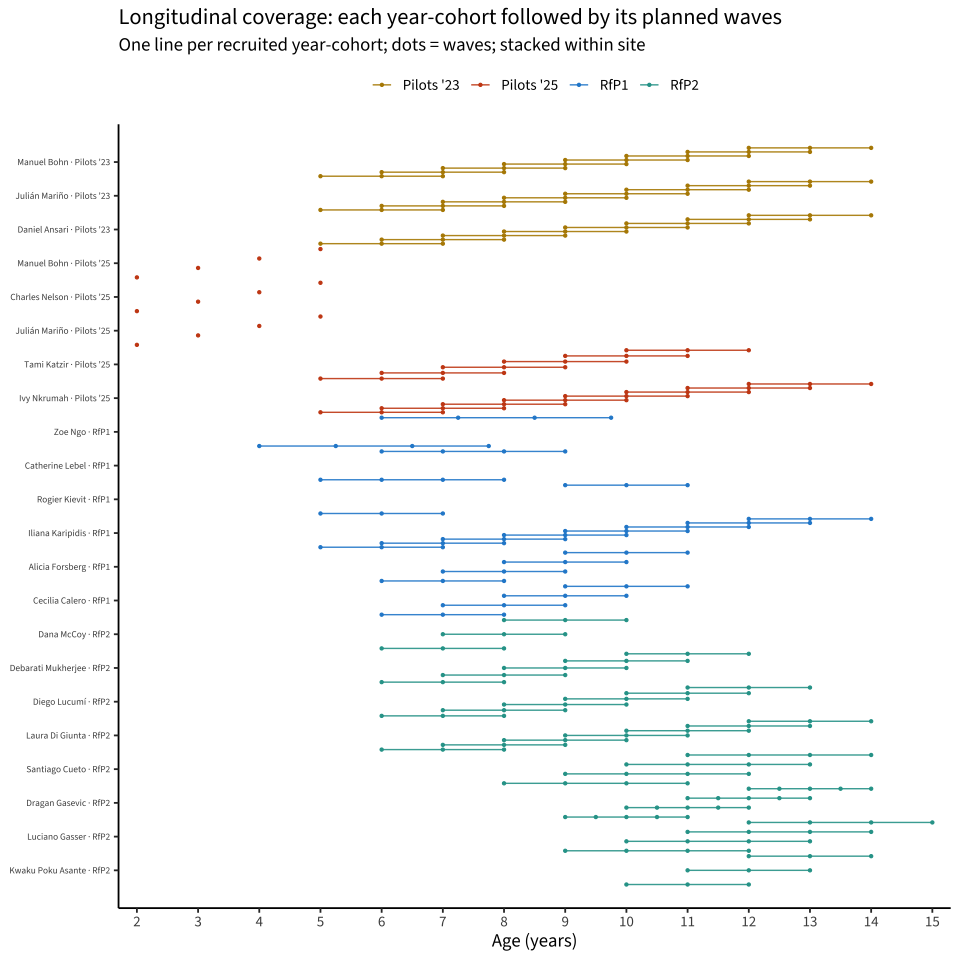
coh2 |>
  reframe(age = seq(floor(x_start), floor(x_end)), .by = c(label, enroll_age, x_start, x_end)) |>
  filter(age >= x_start, age <= x_end) |>
  count(age, name = "n_cohorts") |>
  ggplot(aes(age, n_cohorts)) +
  geom_col(fill = "#268bd2") +
  scale_x_continuous(breaks = 0:16) +
  labs(x = "Age (years)", y = "# year-cohorts covering age",
       title = "Marginal coverage density (sum of the stacked lines above)")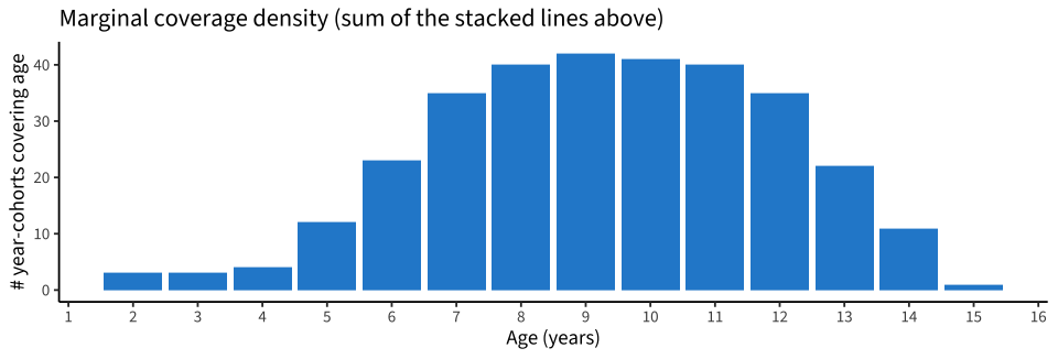
The accumulated waves cover roughly ages 2–15, with the densest coverage in the 6–11 school-age range, where the pilots, RfP1, and RfP2 longitudinal sites pile up. Coverage thins at the early-childhood end (2–5) — carried by only the 2025 pilots and Lebel — and at the older end (13+), which rests on a handful of cohorts aging out of the school-age sites. This is the empirical case for RfP3’s downward-extension priority.
papers/). Ages are the annex cards’ “Age range”; wave schedules are the cohort tables’ “Timeline” column. Where they disagreed we used the more specific value and flagged it in notes (Forsberg, Gasser, Lebel, Calero).n_waves at its cadence. For accelerated-longitudinal sites whose documented age range already spans some follow-up years, this projects each year in the band forward independently and so over-states the upper extent — read the right-hand tails as an upper bound, not a commitment.09_site_coverage.csv for reuse.