05 — Battery design: how short can the battery be and still recover the factors?
ImportantAI-generated — not for publication
The code and prose in this chapter were written by Claude Code (an AI coding agent) under human direction. They have not been line-by-line verified by a human and must not be published or cited as-is.
WarningPreliminary & unvetted analysis
These are exploratory analyses of preliminary, in-progress LEVANTE data. Results have not been reviewed or validated and require checking by the LEVANTE Data Coordinating Center before any use.
The question
03–04 established that the core battery measures a strong, highly-correlated factor structure. That has a practical payoff: if the constructs overlap heavily, we should be able to recover each child’s factor scores from a shorter battery. This notebook quantifies that trade-off.
We combine three ingredients —
the calibrated measurement model (the theory-driven factor structure),
each task’s marginal reliability, and
each task’s administration time (newest = adaptive version where one exists) —
and ask, for any subset of tasks: how well does it recover the factor scores, and how many minutes does it cost? We then read off three battery versions (full / minor reduction / minimal) and the efficient frontier between them.
Per the design brief we target two theory-driven structures (MEFS is already cut, so it does not appear):
2-factor: a fluid / nonverbal factor (matrix, mental rotation, math, hearts & flowers, memory, same-&-different) and a verbal / literacy factor (TROG, vocab, ToM, ROAR word/sentence/phoneme). Note TROG is placed with language here, on theory grounds, despite loading with fluid in 04’s EFA.
4-factor: reasoning / executive function / language / reading.
“Recovery” = factor-score determinacy: the correlation between the factor score estimated from the administered subset and the true latent factor. We calibrate the measurement model once on the full battery, then evaluate every subset against that fixed calibration — exactly how one would design a short form.
Code
source(here::here("common.R"))library(lavaan) # NB: do not attach MASS — it masks dplyr::select; use MASS::mvrnorm qualifiedsc <-read_rds(here("data/scores_all_sites.rds"))sites4 <-c("pilot_mpieva_de_main","pilot_uniandes_co_bogota","pilot_uniandes_co_rural","pilot_western_ca_main")tasks12 <-tibble(short =c("matrix","mrot","math","hf","mg","sds","trog","vocab","tom","swr","sre","pa"),task_id =c("matrix-reasoning","mental-rotation","egma-math","hearts-and-flowers","memory-game","same-different-selection","trog","vocab","theory-of-mind","swr","sre","pa"),f4 =c("reasoning","reasoning","reasoning","ef","ef","ef","language","language","language","reading","reading","reading"),f2 =c("fluid","fluid","fluid","fluid","fluid","fluid","verbal","verbal","verbal","verbal","verbal","verbal"))# tasks with an adaptive version → use ONLY adaptive runs (the newest/deployed form)adaptive_capable <-c("egma-math","matrix-reasoning","mental-rotation","same-different-selection","trog","vocab")# analysis sample: first observation per child per task, 4 data-rich sites,# restricted to the newest (adaptive) version where one exists.fo <- sc |>filter(dataset %in% sites4, task_id %in% tasks12$task_id, !is.na(score)) |>filter(!(task_id %in% adaptive_capable) | adaptive) |>group_by(user_id, task_id) |>arrange(age) |>slice(1) |>ungroup()
1. Ingredients
Marginal reliability
Empirical (marginal) reliability per task from the EAP standard errors, ρ = Var(θ̂) / [Var(θ̂) + mean(SE²)], computed on the deployed-version runs.
Code
rel <- fo |>group_by(short) |>summarise(rel =var(score) / (var(score) +mean(score_se^2, na.rm =TRUE)),.groups ="drop")# sre is a guessing-adjusted *count* score (no model SE) → reliability not# estimable from SE; its odd/even split-half is inflated by speededness, so we# leave it blank and let sre enter the recovery model through its loading only.rel |>right_join(tasks12 |>select(short), by ="short") |>arrange(rel) |>mutate(rel =round(rel, 3)) |> knitr::kable(caption ="Marginal reliability (deployed-version runs; sre = NA, count-based score)")
Reliabilities run from ~0.72 (matrix, ToM) to ~0.93 (ROAR-Word, math). Same & Different is the weakest (~0.62) — its adaptive version has few runs so far (n≈80) and its scoring is still being revised, so treat that number as provisional.
Administration time
Median wall-clock duration per run (newest/adaptive version), robust to the occasional paused-and-resumed session. This is approximate seat time — it includes instructions and natural pauses, so it is an upper-ish estimate of active testing time.
Median administration time (full battery = 54.8 min)
short
minutes
tom
9.4
swr
7.7
math
6.3
matrix
5.3
pa
4.2
mg
4.0
trog
3.8
vocab
3.6
mrot
3.2
sre
3.0
hf
2.9
sds
1.5
ToM is by far the longest (≈10 min — it has spoken-story stimuli); ROAR-Word (≈8 min, 120 quick items) is next. The full 12-task battery runs ≈ 55 min (2026-08 durations; ≈59 min in the June render).
The calibrated measurement model
Two CFAs (FIML, pooled across the four sites, scores standardized within task). We extract the standardized loadings and factor correlations — the fixed calibration that every candidate battery is scored against.
Both models fit well (2-factor CFI = 0.897, 4-factor CFI = 0.915). The factor correlations are high — in the 4-factor model reasoning and EF are almost the same factor (r = 0.97); fluid–verbal in the 2-factor model is r = 0.96. (The pooled FIML fit carries a thin-coverage caveat from Bogotá’s partial battery; per-site structure in 03–04 replicates these loadings, so they are an adequate design calibration.)
2. Recovery metric, and a simulation check
For an administered subset B, factor-score determinacy is computed from the calibrated loadings Λ and factor correlation Φ (restricted to B): the model-implied indicator correlation is Σ = ΛΦΛ′ (unit diagonal), the regression score weights are W = ΦΛ′Σ⁻¹, and the determinacy for factor j is the √ of the j-th diagonal of ΦΛ′Σ⁻¹ΛΦ. A factor with no administered indicator cannot be recovered.
Code
determinacy <-function(Lam, Phi, keep){ L <- Lam[keep, , drop =FALSE]if (any(colSums(abs(L) >0) <1)) return(setNames(rep(NA, ncol(Lam)), colnames(Lam))) S <- L %*% Phi %*%t(L); diag(S) <-1 M <- Phi %*%t(L) %*%solve(S) %*% L %*% PhisetNames(sqrt(pmin(diag(M) /diag(Phi), 1)), colnames(Lam))}
To confirm this analytic quantity really is the recovered-score correlation, we simulate: draw 50,000 children from the calibrated 4-factor model, generate task scores with the model’s loadings + uniquenesses, estimate factor scores from a subset using the regression weights, and correlate with the true latent scores.
The simulation reproduces the analytic determinacy to three decimals, so we use the (exact, instant) analytic version for the frontier below.
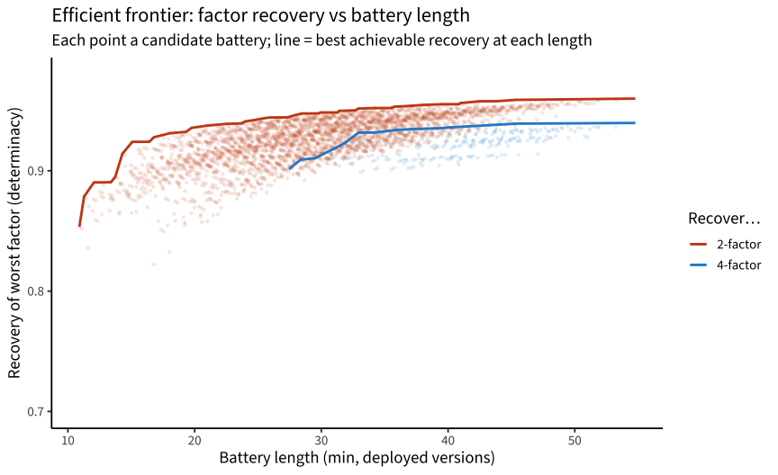
3. The length / recovery frontier
We enumerate every subset of the 12 tasks, compute its total minutes and its recovery of each factor, and keep the worst-recovered factor as the binding constraint. Deployable 4-factor batteries need ≥ 2 indicators per factor.
bind_rows( res |>filter(ind4 >=2) |>transmute(minutes, recovery = det4_min, target ="4-factor"), res |>filter(ind2 >=2) |>transmute(minutes, recovery = det2_min, target ="2-factor")) |>ggplot(aes(minutes, recovery, color = target)) +geom_point(alpha =0.10, size =0.7) +geom_line(data =bind_rows(front4 |>transmute(minutes, recovery = det4_min, target ="4-factor"), front2 |>transmute(minutes, recovery = det2_min, target ="2-factor")),linewidth =1) +scale_color_manual(values =c("4-factor"="#268bd2", "2-factor"="#cb4b16"), name ="Recover…") +scale_x_continuous(breaks =seq(0, 60, 10)) +labs(x ="Battery length (min, deployed versions)",y ="Recovery of worst factor (determinacy)",title ="Efficient frontier: factor recovery vs battery length",subtitle ="Each point a candidate battery; line = best achievable recovery at each length") +coord_cartesian(ylim =c(0.7, 0.98))
The frontier is steep then flat: recovery climbs fast over the first ~30 minutes and then barely improves — going from 30 to 55 minutes buys < 0.04 in determinacy. The 2-factor (broad) target sits well above the 4-factor target, so if only the fluid/verbal split is needed the battery can be far shorter.
Full (12 tasks, ~55 min). Recovers all four factors at 0.94–0.96.
Minor reduction (10 tasks, ~44 min, 74% of the time). Drops ToM (the single longest task, ≈10 min) and Same & Different (longest-running EF task with the weakest, still-provisional scoring). Recovery essentially unchanged (0.93–0.96): ToM’s factor (language) still has TROG + vocab, and EF still has H&F + memory.
Minimal (8 tasks, ~31 min, 52% of the time). The smallest battery that keeps two indicators per 4-factor construct. Recovery 0.91–0.95 — reading takes the largest hit (0.94→0.91) because dropping ROAR-Word leaves the two efficiency/phoneme measures. Halves administration time for ≈0.03 loss.
Broad screen (4 tasks, ~14 min, 26% of the time). If only the fluid vs verbal distinction is needed, four tasks recover both broad factors at ≈0.90 — a viable rapid screener. (2026-08 note: with the updated durations/reliabilities the frontier now picks math + sds + sre + vocab; the June render picked hf instead of sds. Treat the sds slot with caution — its scoring is still provisional — hf’s screener was within a hair of the frontier and is the safer deployment choice.)
What each task buys (leave-one-out)
Dropping a task from the full battery, ranked by recovery lost per minute saved — the cheapest-to-drop tasks are at the top.
Leave-one-out value: recovery lost per minute saved (top = most droppable)
task
minutes_saved
recovery_loss
loss_per_min
tom
9.4131
0.0006
0.0001
matrix
5.3243
0.0031
0.0006
mrot
3.2260
0.0032
0.0010
pa
4.2349
0.0044
0.0010
hf
2.8554
0.0033
0.0011
sre
2.9812
0.0036
0.0012
vocab
3.5564
0.0051
0.0014
math
6.2511
0.0107
0.0017
sds
1.5129
0.0035
0.0023
mg
3.9684
0.0109
0.0027
trog
3.7560
0.0120
0.0032
swr
7.6749
0.0260
0.0034
ToM and matrix-reasoning are the most droppable (long and/or redundant); vocab, TROG, ROAR-Word and math are the most valuable per minute — they anchor the factors (language, reading) that have the fewest strong indicators.
The heavy intercorrelation among constructs (03–04) is exactly what makes the battery compressible: factor scores can be recovered from far fewer tasks than the full battery, because the remaining tasks borrow strength through the factor correlations.
You can cut administration time roughly in half (59 → ~31 min) and still recover every construct at ≈ 0.91–0.95. Dropping just ToM and Same & Different (→ ~44 min) costs almost nothing.
The binding constraint is reading, not the fluid core: reasoning, EF and the broad fluid factor stay > 0.93 even in short batteries, because reasoning ≈ EF and they pool. Reading is the factor to protect when trimming — keep ROAR-Word if reading scores matter.
For triage/screening where only the broad fluid/verbal split is needed, a ~14-minute four-task screener recovers both factors at ≈ 0.90.
Caveats. Durations are median wall-clock (include instructions/pauses) for the deployed adaptive versions; composition-only — we did not model shortening tasks within themselves (CAT stopping rules), which could shave more time. The calibration is pooled pilot-site data with thin Bogotá coverage; Same & Different’s reliability/scoring is provisional; sre enters via its loading (no model-based reliability). Recovery is of the factor scores, not of every task’s specific variance — a minimal battery measures the constructs, not the individual tasks.