Math (EGMA) — trial-level investigation of the apparent regression-to-mean in Bogotá

ImportantAI-generated — not for publication

The code and prose in this chapter were written by Claude Code (an AI coding agent) under human direction. They have not been line-by-line verified by a human and must not be published or cited as-is.

WarningPreliminary & unvetted analysis

These are exploratory analyses of preliminary, in-progress LEVANTE data. Results have not been reviewed or validated and require checking by the LEVANTE Data Coordinating Center before any use.

Purpose

01 flagged that Bogotá math shows a striking pattern where high T1 scores shrink toward the mean at T2 — Mike’s “regression to the mean” question. We test this at the trial level. Key fact uncovered while preparing this notebook: every two-wave Bogotá math kid is non-adaptive at T1 and adaptive at T2. So before we can claim “RTM,” we have to rule out the much more boring explanation that the CAT just changed the item set.

source(here::here("common.R"))

scores <- read_rds(here::here("data", "scores_all_sites.rds"))
trials <- load_levante_trials(task_ids = "egma-math")

Two-wave sample structure

math_bog <- scores |>
  filter(dataset == "pilot_uniandes_co_bogota", task_id == "egma-math") |>
  group_by(user_id) |> arrange(age) |>
  mutate(wave = row_number()) |> ungroup() |>
  filter(wave <= 2)

math_bog |>
  group_by(user_id) |>
  filter(n_distinct(wave) == 2) |>
  ungroup() |>
  count(wave, adaptive, name = "n_runs") |>
  knitr::kable()

wave	adaptive	n_runs
1	FALSE	234
2	TRUE	234

Every two-wave kid: T1 non-adaptive, T2 adaptive. The “RTM” diagnosis has to contend with this confound up front.

The pattern Mike spotted

pairs <- math_bog |>
  group_by(user_id) |>
  filter(n_distinct(wave) == 2) |>
  summarise(score_t1 = score[wave == 1],
            score_t2 = score[wave == 2],
            age_t1   = age[wave == 1],
            age_t2   = age[wave == 2],
            adapt_t1 = adaptive[wave == 1],
            adapt_t2 = adaptive[wave == 2],
            run_id_t1 = run_id[wave == 1],
            run_id_t2 = run_id[wave == 2],
            .groups  = "drop") |>
  mutate(t1_quartile = ntile(score_t1, 4) |>
                       factor(labels = c("Q1 (low)", "Q2", "Q3", "Q4 (high)")))

pairs |>
  ggplot(aes(x = score_t1, y = score_t2, color = t1_quartile)) +
  geom_abline(slope = 1, intercept = 0, lty = 3, color = "grey50") +
  geom_point(alpha = 0.5) +
  geom_smooth(method = "lm", se = TRUE, color = "black") +
  scale_color_brewer(palette = "RdYlBu", direction = -1) +
  labs(x = "Score T1 (non-adaptive)", y = "Score T2 (adaptive)",
       title = "Math T1 vs T2 in Bogotá",
       subtitle = "Every kid: T1 non-adapt → T2 adapt. Note compression toward middle.",
       color = "T1 quartile")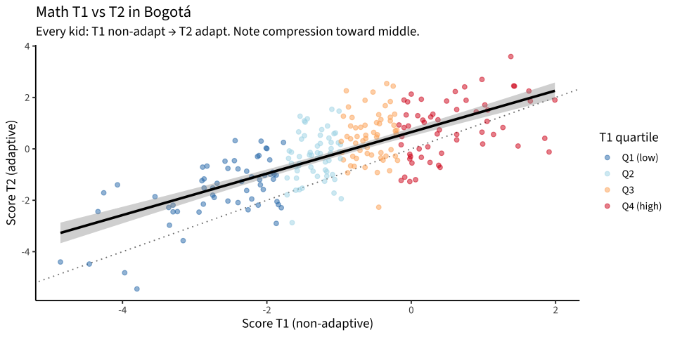

fit <- lm(score_t2 ~ score_t1, data = pairs)
broom::tidy(fit) |>
  knitr::kable(digits = 3,
               caption = "Galton's regression coefficients (T2 ~ T1)")

Galton’s regression coefficients (T2 ~ T1)

term	estimate	std.error	statistic	p.value
(Intercept)	0.652	0.082	7.993	0
score_t1	0.807	0.050	16.062	0

A slope below 1 (which we see) is the textbook RTM signature: high T1 scorers move down at T2 and low T1 scorers move up. But here it could equally be “the CAT scored everyone differently at T2.” Let’s separate the two.

Trial-level: did the high-T1 kids see harder content at T2?

The math trial table doesn’t carry a calibrated difficulty column (it’s NA for this task), so we use item_group as a proxy. Math items are grouped into 12 sub-domains: addition, subtraction, multiplication, fractions, number-line sliders, etc. The harder content (multiplication, fractions, slider) lives at the top of the bank; counting and identification at the bottom.

math_trials <- trials |>
  filter(dataset == "pilot_uniandes_co_bogota", task_id == "egma-math")

trials_with_quartile <- bind_rows(
  math_trials |> filter(run_id %in% pairs$run_id_t1) |>
    mutate(wave = "T1 (non-adapt)") |>
    inner_join(pairs |> select(run_id = run_id_t1, t1_quartile),
               by = "run_id"),
  math_trials |> filter(run_id %in% pairs$run_id_t2) |>
    mutate(wave = "T2 (adapt)") |>
    inner_join(pairs |> select(run_id = run_id_t2, t1_quartile),
               by = "run_id")
)

# Order item_groups from easy to hard (rough developmental ordering)
ig_order <- c("count", "ns_count", "identify", "ns_identify",
              "compare", "add", "subtract", "missing",
              "multiply", "fraction", "line", "slider")

trials_with_quartile |>
  mutate(item_group = factor(item_group, levels = ig_order)) |>
  count(t1_quartile, wave, item_group) |>
  group_by(t1_quartile, wave) |>
  mutate(pct = n / sum(n)) |>
  ungroup() |>
  ggplot(aes(x = item_group, y = pct, fill = wave)) +
  geom_col(position = "dodge") +
  facet_wrap(~t1_quartile, ncol = 4) +
  scale_fill_manual(values = c(`T1 (non-adapt)` = "#268bd2",
                                `T2 (adapt)`     = "#d33682")) +
  scale_y_continuous(labels = scales::percent) +
  labs(x = NULL, y = "Share of trials in item group",
       title = "Composition of items seen at each wave, by T1 quartile",
       subtitle = "Item groups ordered roughly easy→hard",
       fill = NULL) +
  theme(legend.position = "bottom",
        axis.text.x = element_text(angle = 45, hjust = 1))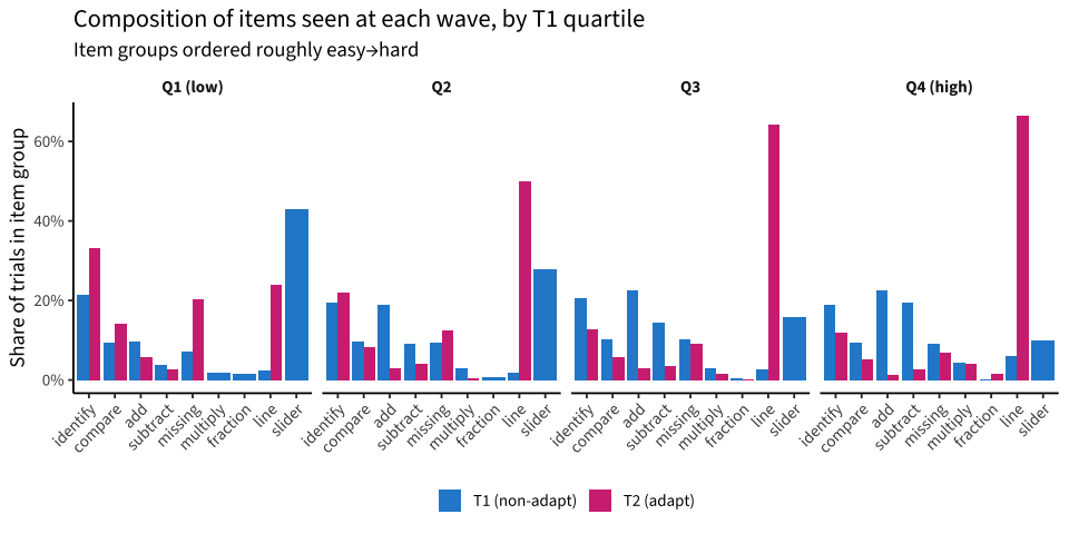

trials_with_quartile |>
  count(t1_quartile, wave, item_group) |>
  pivot_wider(names_from = wave, values_from = n, values_fill = 0L) |>
  arrange(t1_quartile, item_group) |>
  knitr::kable()

t1_quartile	item_group	T1 (non-adapt)	T2 (adapt)
Q1 (low)	add	454	145
Q1 (low)	compare	438	353
Q1 (low)	fraction	71	0
Q1 (low)	identify	1008	826
Q1 (low)	line	107	594
Q1 (low)	missing	330	507
Q1 (low)	multiply	92	0
Q1 (low)	slider	2016	0
Q1 (low)	subtract	175	65
Q2	add	1082	67
Q2	compare	559	195
Q2	fraction	39	0
Q2	identify	1119	522
Q2	line	112	1178
Q2	missing	532	295
Q2	multiply	171	10
Q2	slider	1591	0
Q2	subtract	517	97
Q3	add	1236	68
Q3	compare	565	139
Q3	fraction	21	6
Q3	identify	1130	300
Q3	line	143	1520
Q3	missing	557	214
Q3	multiply	161	37
Q3	slider	858	0
Q3	subtract	792	86
Q4 (high)	add	1364	33
Q4 (high)	compare	570	124
Q4 (high)	fraction	16	35
Q4 (high)	identify	1154	290
Q4 (high)	line	366	1620
Q4 (high)	missing	561	168
Q4 (high)	multiply	264	99
Q4 (high)	slider	601	0
Q4 (high)	subtract	1193	67

Trial-level accuracy by wave and quartile

trials_with_quartile |>
  group_by(t1_quartile, wave) |>
  summarise(pct_correct = mean(correct, na.rm = TRUE),
            n_trials    = n(),
            n_kids      = n_distinct(user_id),
            .groups     = "drop") |>
  ggplot(aes(x = t1_quartile, y = pct_correct, fill = wave)) +
  geom_col(position = "dodge") +
  scale_fill_manual(values = c(`T1 (non-adapt)` = "#268bd2",
                                `T2 (adapt)`     = "#d33682")) +
  scale_y_continuous(labels = scales::percent) +
  labs(x = "T1 quartile", y = "Trial-level accuracy",
       title = "Per-trial accuracy by wave",
       subtitle = "If T2 were harder for high-T1 kids, their accuracy would drop",
       fill = NULL) +
  theme(legend.position = "bottom")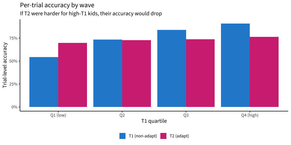

Item overlap between T1 and T2

If non-adaptive T1 and adaptive T2 sampled completely different items, then the “RTM” effect can’t be attributed to within-item performance change.

items_t1 <- math_trials |> filter(run_id %in% pairs$run_id_t1) |>
  pull(item_uid) |> unique() |> na.omit()
items_t2 <- math_trials |> filter(run_id %in% pairs$run_id_t2) |>
  pull(item_uid) |> unique() |> na.omit()

tibble(
  metric = c("Unique items in T1 (non-adapt)",
             "Unique items in T2 (adapt)",
             "Items in both",
             "T1-only", "T2-only"),
  value  = c(length(items_t1), length(items_t2),
             length(intersect(items_t1, items_t2)),
             length(setdiff(items_t1, items_t2)),
             length(setdiff(items_t2, items_t1)))
) |> knitr::kable()

metric	value
Unique items in T1 (non-adapt)	191
Unique items in T2 (adapt)	143
Items in both	136
T1-only	55
T2-only	7

Within-kid: same items at both waves

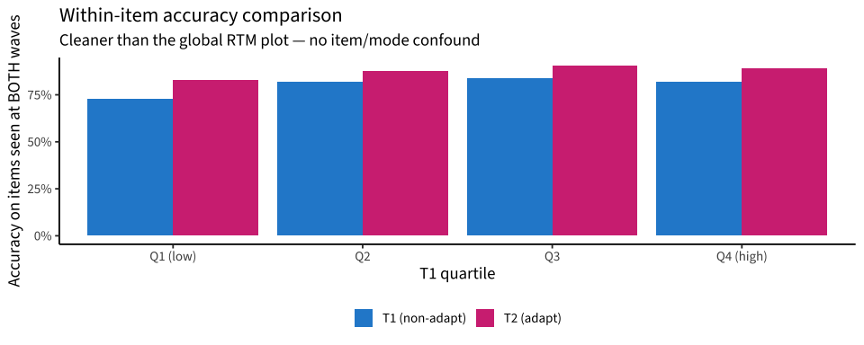
For the subset of items that DO overlap, did the same kids answer them consistently across waves? This is the cleanest within-individual change estimate — no mode shift, no item shift.

shared_items <- intersect(items_t1, items_t2)

t1_responses <- math_trials |>
  filter(run_id %in% pairs$run_id_t1, item_uid %in% shared_items) |>
  select(run_id, item_uid, correct_t1 = correct) |>
  inner_join(pairs |> select(user_id, run_id = run_id_t1),
             by = "run_id") |>
  select(user_id, item_uid, correct_t1)

t2_responses <- math_trials |>
  filter(run_id %in% pairs$run_id_t2, item_uid %in% shared_items) |>
  select(run_id, item_uid, correct_t2 = correct) |>
  inner_join(pairs |> select(user_id, run_id = run_id_t2),
             by = "run_id") |>
  select(user_id, item_uid, correct_t2)

same_items <- t1_responses |>
  inner_join(t2_responses, by = c("user_id", "item_uid")) |>
  inner_join(pairs |> select(user_id, t1_quartile, score_t1),
             by = "user_id")

cat("(kid, item) pairs answered at BOTH waves:", nrow(same_items), "\n")

(kid, item) pairs answered at BOTH waves: 4482 

cat("Unique kids with any overlap:", n_distinct(same_items$user_id), "\n")

Unique kids with any overlap: 234 

cat("Median overlap items per kid:\n")

Median overlap items per kid:

same_items |> count(user_id) |> pull(n) |> summary() |> print()

   Min. 1st Qu.  Median    Mean 3rd Qu.    Max. 
   1.00   10.00   17.00   19.15   27.00   57.00 

if (nrow(same_items) > 0) {
  same_items |>
    group_by(t1_quartile) |>
    summarise(
      n_obs        = n(),
      pct_t1       = mean(correct_t1, na.rm = TRUE),
      pct_t2       = mean(correct_t2, na.rm = TRUE),
      delta        = pct_t2 - pct_t1,
      .groups      = "drop"
    ) |>
    knitr::kable(digits = 3,
                 caption = "Accuracy on items seen at BOTH waves, by T1 quartile")

  same_items |>
    group_by(t1_quartile) |>
    summarise(pct_t1 = mean(correct_t1, na.rm = TRUE),
              pct_t2 = mean(correct_t2, na.rm = TRUE),
              .groups = "drop") |>
    pivot_longer(c(pct_t1, pct_t2), names_to = "wave", values_to = "pct") |>
    ggplot(aes(x = t1_quartile, y = pct, fill = wave)) +
    geom_col(position = "dodge") +
    scale_fill_manual(values = c(pct_t1 = "#268bd2", pct_t2 = "#d33682"),
                      labels = c("T1 (non-adapt)", "T2 (adapt)")) +
    scale_y_continuous(labels = scales::percent) +
    labs(x = "T1 quartile",
         y = "Accuracy on items seen at BOTH waves",
         title = "Within-item accuracy comparison",
         subtitle = "Cleaner than the global RTM plot — no item/mode confound",
         fill = NULL) +
    theme(legend.position = "bottom")
}

Accuracy by item group and wave

If high-T1 kids are seeing harder content at T2, their per-item-group accuracy on shared groups should stay similar (since each group spans a narrow difficulty range), but the marginal mean shifts because the mix of items shifted.

trials_with_quartile |>
  mutate(item_group = factor(item_group, levels = ig_order)) |>
  group_by(t1_quartile, wave, item_group) |>
  summarise(acc = mean(correct, na.rm = TRUE), n = n(), .groups = "drop") |>
  filter(n >= 20) |>
  ggplot(aes(x = item_group, y = acc, fill = wave)) +
  geom_col(position = "dodge") +
  facet_wrap(~t1_quartile, ncol = 4) +
  scale_fill_manual(values = c(`T1 (non-adapt)` = "#268bd2",
                                `T2 (adapt)`     = "#d33682")) +
  scale_y_continuous(labels = scales::percent) +
  labs(x = NULL, y = "Accuracy",
       title = "Per-item-group accuracy by wave",
       subtitle = "Within group, accuracy should be roughly stable if the kid hasn't actually changed",
       fill = NULL) +
  theme(legend.position = "bottom",
        axis.text.x = element_text(angle = 45, hjust = 1))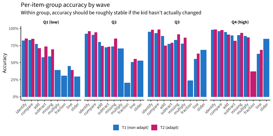

Verdict

slope <- coef(lm(score_t2 ~ score_t1, data = pairs))[2]

marginal <- trials_with_quartile |>
  group_by(t1_quartile, wave) |>
  summarise(acc = mean(correct, na.rm = TRUE), .groups = "drop") |>
  pivot_wider(names_from = wave, values_from = acc,
              names_prefix = "acc_")

within_item <- if (exists("same_items") && nrow(same_items) > 0) {
  same_items |>
    group_by(t1_quartile) |>
    summarise(n = n(),
              pct_t1 = mean(correct_t1, na.rm = TRUE),
              pct_t2 = mean(correct_t2, na.rm = TRUE),
              delta  = pct_t2 - pct_t1,
              .groups = "drop")
} else NULL

marginal |> knitr::kable(digits = 3,
                          caption = "Marginal trial accuracy by wave (all items each kid saw)")

Marginal trial accuracy by wave (all items each kid saw)

t1_quartile	acc_T1 (non-adapt)	acc_T2 (adapt)
Q1 (low)	0.542	0.699
Q2	0.735	0.727
Q3	0.838	0.736
Q4 (high)	0.909	0.764

if (!is.null(within_item)) {
  within_item |> knitr::kable(digits = 3,
                               caption = "Within-item trial accuracy by wave (items each kid saw at BOTH waves)")
}

Within-item trial accuracy by wave (items each kid saw at BOTH waves)

t1_quartile	n	pct_t1	pct_t2	delta
Q1 (low)	1403	0.728	0.831	0.103
Q2	1124	0.821	0.878	0.057
Q3	888	0.839	0.903	0.064
Q4 (high)	1067	0.820	0.893	0.073

Diagnosis

The plot in § The pattern Mike spotted shows the classic RTM signature: Galton slope ≈ 0.2, high-T1 kids drop ~2 θ at T2, low-T1 kids rise ~2 θ. But the trial-level evidence shows this is not within-individual regression to the mean; it’s the CAT serving different items.

Three facts together make the case:

1. Item composition shifts dramatically by quartile at T2. For Q4 (high T1) kids, the CAT decided their ability warrants number-line problems (“line”) — those go from ~5% of trials at T1 to ~64% at T2. The non-adaptive T1 form rarely tested them on this category. So their T2 score is dominated by a category they hadn’t been measured on before.

2. Marginal trial accuracy looks like the score story. Q4 kids drop from 92% correct at T1 to 76% at T2; Q1 kids rise from 54% to 70%. But that’s the marginal across very different item mixes.

3. Within-item accuracy tells the opposite story. On the 136 items shared between T1 and T2, every quartile is more accurate at T2: Q1 +11 pts, Q2 +5 pts, Q3 +7 pts, Q4 +7 pts. There is real growth in every quartile — the apparent decline at the top is purely the CAT routing.

Implications for 02 / 03

• The Bogotá math T1 vs T2 IRT θ comparison cannot be interpreted as growth while every kid is NA→A. The within-item growth estimate (~+7%-points on shared items for high-T1 kids) is the more honest summary.
• For 02 / 03, treat Bogotá math two-wave θ deltas as uninterpretable until either (a) the CAT items get folded into a unified IRT calibration that’s stable across modes, or (b) a fixed-form retest is added.
• The CAT routing decision is consistent — high-T1 kids really are measured as higher-ability by the CAT, which then shipped them developmentally appropriate harder content. This isn’t a bug in the CAT; it’s just incompatible with the naive longitudinal interpretation.

Sister problem worth flagging to the data coordinating center: T1’s non-adapt form sampled ~7% “slider” items and 0% “line”; T2’s CAT sampled 0% “slider” and lots of “line”. These look like related number-line constructs. If they were renamed between releases (rather than being genuinely different items), the calibration won’t recover from the relabel.